Swarming Itokawa with cubesats#
In this example we consider a rather advanced mission option inspired to us by the European Space Agency HERA mission. HERA is an interplanetary spacecraft that will explore the binary system named Didymos in 2025. In the case of HERA, two cubesats called Milani and Juventas, will detach from the main mother satellite to perform some detailed exploration of the system, including the exploartion of its gravity field. The use of cubesats to increase the mission scientific output, while minimizing risks connected to operating in a highly unknown environment, is being considered as an option for several advanced missions.
We will show the use of cascade to study the dynamics of a large number of cubesats simultaneously orbiting an irregular body. We will assume a number of cubesats get deployed from a common orbit and compute the \(DV\) needed for such a swarm to avoid collision while keeping all the cubesats within some maximum and minimum range from the asteroid centre.
Note
This example concerns a case that has not driven the development of cascade. In particular, the events frequency (collision reentry and exit) is much higher if compared to the optimal timestep of Taylor integrator. As a consequence the overall algorithm, still very usable, becomes less efficient as dynamics computations (i.e. the Taylor coefficients) are thrown away at each event trigger.
Let us start with some imports:
# core imports
import pykep as pk
import numpy as np
import scipy
import pickle as pkl
import cascade as csc
import heyoka as hy
from copy import deepcopy

# plotting
from mpl_toolkits.mplot3d import Axes3D
from matplotlib import pyplot as plt
%matplotlib inline
Importing and defining the irregular body#
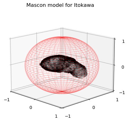
In the example we are going to consider the asteroid Itokawa. We will use mascons to have a representation of irregular bodies. In other words, Itokawa will be modelled as set of point masses located in specific positions and with some given mass.
with open("data/itokawa_mascon.pk", "rb") as file:
    mascon_points, mascon_masses, name = pkl.load(file)
print(name+":", "number of mascons is", len(mascon_masses))
Itokawa: number of mascons is 41748
In the case of Itokawa, the mascon model of the body is here provided by the pickled file itokawa_mascon.pk and was developed in the project geodesyNET. This particular mascon model corresponds to a perfectly uniform density asteroid. While Itokawa is actually inhomogeneous, for the purpose of this example a homogenous model can be used too.
Some physical properties of the asteroid are defined next:
L = 350.44 # [m] units of length (used in the mascon model)
M = 3.51E10 # [kg] units of mass (the Itokawa mass)
G = 6.6743E-11 # [m^3/s^2/kg] units for G (the Cavendish constant)
T = np.sqrt(L**3/G/M) # [s] induced units of time
wz = 2*np.pi / (12.132 * 60. * 60. / T) # asteroid angular velocity is 12.132 hours, here computed in the selected units
w_vec = np.array([0., 0., wz]) # we assume a rotation around the z axis
we now visualize the mascon model:
# Define the 3d Axis
fig = plt.figure()
ax = fig.add_subplot(111, projection='3d')

# Plot all mascons
ax.scatter3D(mascon_points[:,0], mascon_points[:,1], mascon_points[:,2], alpha=0.03, s=1, c='k')

# Plot a safety sphere around it
r = np.sqrt(1.1)
u, v = np.mgrid[0:2*np.pi:40j, 0:np.pi:40j]
X = r*np.cos(u)*np.sin(v)
Y = r*np.sin(u)*np.sin(v)
Z = r*np.cos(v)
ax.plot_wireframe(X, Y, Z, color="r", alpha=0.1)

# Set the axis limits
limit=1
ax.set_xlim(-limit,limit)
ax.set_ylim(-limit,limit)
ax.set_zlim(-limit,limit)
ax.view_init(15,-45)
ax.set_title("Mascon model for Itokawa")
ax.set_xticks([-1,0,1])
ax.set_yticks([-1,0,1])
ax.set_zticks([-1,0,1]);
Exploring the dynamics of one single cubesat#
Before delving into a full cascade simulation, it is useful to investigate the dynamics of a single cubesat around the irregular body considered. We will do so using directly heyoka, knowing that cascade smulations also use Taylor integrators for the dynamics provided via heyoka.
In the cascade.dynamics module we provide the dynamics of a spacecraft around a rotating asteroid. Such dynamics implements the following equations of motion:
see the paper Reliable event detection for Taylor methods in astrodynamics for further information. Note that we are using units where \(G=1\) and \(GM=1\).
dyn = csc.dynamics.mascon_asteroid(Gconst = 1., masses=mascon_masses, points=mascon_points, omega = w_vec)
We now instantiate a Taylor integrator using heyoka’s hy.taylor_adaptive class. Note that we have added two terminal events to the equations as to perform a manouvre whenever the spacecarft is too close or too far:
where \(\mathbf {\hat r}\) represents the unit vector of the spacecraft position and \(\mathbf v\) its velocity.
Note how the taylor_adaptive constructor is called with the argument compact_mode set to True as otherwise the equation generation would take a considerable amount of time.
# Re-entry event
safety_radius = 1.1
# Exit event
exit_radius = 3.

x,y,z = hy.make_vars("x", "y", "z")
vx,vy,vz = hy.make_vars("vx", "vy", "vz")

# Applies the DV to the spacecraft state
def dv_invert_radial(ta, mr, d_sgn):
    global DV
    r = deepcopy(ta.state[:3])
    rotv = np.cross(w_vec, r)
    v = deepcopy(ta.state[3:6]) - rotv
    rhat = r / np.linalg.norm(r)
    ta.state[3:6] = v - 2*np.dot(rhat,v) * rhat + rotv
    DV+=np.linalg.norm(2*np.dot(rhat,v) * rhat)
    return True

# Define a terminal event that detects the entry in the safety sphere
reentry_ev = hy.t_event(
        # The event equation.
        x**2+y**2+z**2 - safety_radius**2,
        # The callback.
        callback = dv_invert_radial)

# Define a terminal event that detects the exit from a sphere
exit_ev = hy.t_event(
        # The event equation.
        x**2+y**2+z**2 - exit_radius**2,
        # The callback.
        callback = dv_invert_radial)

# Constructs the Taylor integrator
taylor = hy.taylor_adaptive(sys=dyn, state = [0.,0.,0.,0.,0.,0.], compact_mode=True, t_events=[reentry_ev, exit_ev])
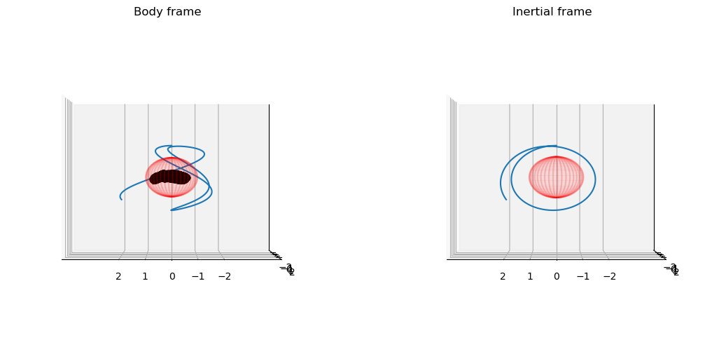
We start simulating the orbit the cubesats will be deployed from. Such an orbit is here designed in the non-rotating frame with an initial position \(\mathbf r_{ic}\) and a circular velocity of magnitude \(\sqrt{\frac{1}{r_ic}}\). The resulting dynamics is very sensitive to these choices, given the irregular form of the body and the close proximity to the asteroid.
# This is a phase we can use to design the starting orbit
theta = 2*np.pi * 0/50
cs = np.cos(theta)
sn = np.sin(theta)
# We consider a polar orbit with velocity aligned to the x axis
r_ic = np.array([0., 1.7*sn, 1.7*cs])
vrot = np.cross(w_vec, r_ic)
v_ic = np.array([np.sqrt(1./np.linalg.norm(r_ic))*cs, 0., -np.sqrt(1./np.linalg.norm(r_ic))*sn]) - vrot
taylor.state[:3] = r_ic
taylor.state[3:6] = v_ic
taylor.time=0.
# The propagation time correspond to roughly 24 hours (i.e. roughly two Itokawa rotations)
tgrid = np.linspace(0., 2*10.19, 1000)
# Global DV in case manouvres are done
DV=0
We perform the numerical propagation.
Tip
The use of the propagate_grid method of heyoka’s Taylor integrator, in this case will ensure we are able to plot the entire trajectory at the end, while sacrificing performances only marginally.
mother = taylor.propagate_grid(tgrid)
The “mother” trajectory#
We now first plot the cubesat trajectory, then compute the control DV that is needed (if any) to keep the cubesat within the desired range from the asteroid.
# This helper function can be used to transform the simulation output into the inertial frame
def rotate(tgrid, states, w_vec):
    from scipy.spatial.transform import Rotation as rot
    import numpy as np
    from copy import deepcopy
    retval = deepcopy(states)
    direction = w_vec
    for t, item in zip(tgrid, retval):
        R = rot.from_rotvec(t * direction).as_matrix()
        item[:3] = R@item[:3]
        item[3:6] = R@item[3:6]
    return retval
mother_rotated=rotate(tgrid, mother[4], w_vec)
# Define the 3d Axis
fig = plt.figure(figsize = (13,7))

#Plot in the rotatting frame
ax = fig.add_subplot(121, projection='3d')

# Plot all mascons
ax.scatter3D(mascon_points[:,0], mascon_points[:,1], mascon_points[:,2], alpha=0.05, s=2, c='k')

# Plot the safety sphere around it
r = np.sqrt(1.1)
u, v = np.mgrid[0:2*np.pi:40j, 0:np.pi:40j]
X = r*np.cos(u)*np.sin(v)
Y = r*np.sin(u)*np.sin(v)
Z = r*np.cos(v)
ax.plot_wireframe(X,Y,Z, color="r", alpha=0.1)

ax.plot3D(mother[4][:,0],mother[4][:,1],mother[4][:,2])

limit=4
ax.set_xlim(-limit,limit)
ax.set_ylim(-limit,limit)
ax.set_zlim(-limit,limit)
ax.view_init(0,90)
ax.set_title("Body frame")
ax.set_xticks([-2, -1,0,1, 2])
ax.set_yticks([-2, -1,0,1, 2])
ax.set_zticks([])

# Plot in the inertial frame
ax = fig.add_subplot(122, projection='3d')
# Plot the safety sphere around it
r = safety_radius
u, v = np.mgrid[0:2*np.pi:40j, 0:np.pi:40j]
X = r*np.cos(u)*np.sin(v)
Y = r*np.sin(u)*np.sin(v)
Z = r*np.cos(v)
ax.plot_wireframe(X,Y,Z, color="r", alpha=0.1)

ax.plot3D(mother_rotated[:,0],mother_rotated[:,1],mother_rotated[:,2])

limit=4
ax.set_xlim(-limit,limit)
ax.set_ylim(-limit,limit)
ax.set_zlim(-limit,limit)
ax.view_init(0,90)
ax.set_title("Inertial frame")
ax.set_xticks([-2, -1,0,1, 2])
ax.set_yticks([-2, -1,0,1, 2])
ax.set_zticks([]);
In case the cubesat manouvres to keep itself in the desired range we evaluate the amount of DV that is provided by the cubesat propulsion system:
print("Total DV: ", DV * L / T, "m/s")
print("Trajectory duration: ", taylor.time*T/60/60/24, "days")
Total DV:  0.0 m/s
Trajectory duration:  1.0110078428455458 days
in this case zero, but in general not necessarily so.
Simulate cubesat swarming#
Having had a look at the dynamics of a single cubesat, we move on to study the behaviour of a swarm of cubesats under the same dynamics. We assume that each cubesat has the capability to perform manouvres whenever it gets too close to another element of the swarm, to the central body or whenever it flies too far away.
We thus instantiate a cascade.sim object to perform a collision simulation where each body has the same collisional radius. Upon the detection of a collision event we will perfrom an avoidance manouvre.
Upon detection of a reentry or exit event (in this case corresponding to entering the safe sphere) we perform a manouvre to invert the radial component of the velocity.
At the beginning only the mother craft is in the simulation. At each deployment a new cubesat will be co-orbiting the asteroid.
# Number of cubesats to simulate
n_cubesats = 50
# Collisional radius (5m)
radius = 5. / L
# The initial state is the mother only
ic_state = np.ones((1,7)) * radius
ic_state[0][:6] = mother[4][0]
We are now ready to instantiate a cascade simulation. With respect to previous examples we here need to make use of the argument compact_mode else the just in time compilation of the internal Taylor integrators will take too much time. With compact_mode we are sacrificing some optimizations in the jitted code but we allow the simulation object to be built in a few seconds only even if the mascon model has tens of thousands of mascons adding to the right hand side of the dynamics.
We have also set an exit_radius argument as to be able to trigger events when cubesats are going too far from the center and thus keep the entire swarm always close to the asteroid.
# Number of collisional timesteps to be processed in parallel.
n_par_ct = 100
# Timestep of the simulation
simulation_step = 2 * np.pi / 10.
# Collisional timestep
collisional_step = simulation_step / n_par_ct
# Re-entry event
safety_radius = 1.1
# Exit event
exit_radius = 3.
# The simulation object
sim = csc.sim(ic_state, collisional_step, dyn=dyn, reentry_radius=safety_radius, n_par_ct = 100, compact_mode=True, exit_radius = exit_radius)
We now run a simulation where collisions are avoided by a collision avoidance manouvre simulating a virtual elastic collision (and using cubesat \(DV\)) and to remain within the exit and the safety radius (using cubesat \(DV\)).
# Simulation length in time units
final_t = 4 * pk.DAY2SEC / T
# We will store for each cubesat the cumulated DV
DV = np.zeros(n_cubesats)
# Counters
n_coll, n_sm, n_am = 0, 0, 0
# We store the positions of the events
ev_pos = []
# We also store the position of all cubesats at the end of each step
all_pos = deepcopy(ic_state)
counter= 1
# Start of the simulation
while sim.time < final_t:
    # One step
    oc = sim.step()
    if counter<n_cubesats:
        # copying current swarm
        new_ic_state = deepcopy(sim.state)
        # adding one element where the mother is
        new_ic_state = np.concatenate((new_ic_state, [new_ic_state[0]]))
        # adding deployment
        new_ic_state[-1][:3] = new_ic_state[-1][:3] + new_ic_state[-1][:3]/np.linalg.norm(new_ic_state[-1][:3]) * 10/L
        sim.set_new_state_pars(new_ic_state)
        counter+=1

    # Appending the cubesat positions
    all_pos = np.concatenate((all_pos, sim.state))
    # Cleaning the print
    print("\r                                                                              ",end='')
    # Printing time
    print(f"\rTime: {sim.time:3.3f} - cubesats: {counter}", end='')

    # Checking events
    if oc == csc.outcome.collision:
        pi, pj = sim.interrupt_info
        # Collision Avoidance Manouvre
        print(" - CAM:", pi,pj, end='')
        # sat i inertial state
        ri = deepcopy(sim.state[pi][:3])
        vroti =  np.cross(w_vec, ri)
        vi = sim.state[pi][3:6] - vroti
        # sat j inertial state
        rj = deepcopy(sim.state[pj][:3])
        vrotj =  np.cross(w_vec, rj)
        vj = sim.state[pj][3:6] - vrotj
        # Elastic collision: the velocity components along rij are exchanged
        rij = (ri-rj) / np.linalg.norm(ri-rj)
        vi_r = np.dot(vi, rij) * rij
        vj_r = np.dot(vj, rij) * rij
        vi = vi - vi_r + vj_r
        vj = vj - vj_r + vi_r
        # ... in the rotating frame
        sim.state[pi][3:6] = vi + vroti
        sim.state[pj][3:6] = vj + vrotj
        # Updating DVs
        DV_mag = np.linalg.norm(vj_r-vi_r)
        DV[pi]+= DV_mag
        DV[pj]+= DV_mag
        # Updating the number of collisions counter and the event positions
        n_coll+=1
        ev_pos.append(ri)

    if oc == csc.outcome.reentry:
        pi = sim.interrupt_info
        # Safety Manouvre
        print(" - SM:", pi, end='')
        # sat i inertial state
        ri = deepcopy(sim.state[pi][:3])
        vrot = np.cross(w_vec, ri)
        vi = sim.state[pi][3:6] - vrot
        # Inverting the radial inertial velocity component and transforming back to the rotating frame
        hatr = ri / np.linalg.norm(ri)
        sim.state[pi][3:6] = vi - 2*np.dot(hatr,vi) * hatr + vrot
        # Updating DVs
        DV[pi]+=np.linalg.norm(2*np.dot(hatr,vi) * hatr)
        # Updating the number of safety manouvres counter and the event positions
        n_sm+=1
        ev_pos.append(ri)

    if oc == csc.outcome.exit:
        pi = sim.interrupt_info
        # Re-approach Manouvre
        print(" - RAM:", pi, end='')
        # sat i inertial state
        ri = deepcopy(sim.state[pi][:3])
        vrot = np.cross(w_vec, ri)
        vi = sim.state[pi][3:6] - vrot
        # Inverting the radial inertial velocity component and transforming back to the rotating frame
        hatr = ri / np.linalg.norm(ri)
        sim.state[pi][3:6] = vi - 2*np.dot(hatr,vi) * hatr + vrot
        # Updating DVs
        DV[pi]+=np.linalg.norm(2*np.dot(hatr,vi) * hatr)
        # Updating the number of safety manouvres counter and the event positions
        n_am+=1
        ev_pos.append(ri)

ev_pos = np.array(ev_pos)
print("\nNumber of collisions: ", n_coll)
print("Number of safety manouvres: ", n_sm)
print("Number of re-approach manouvres: ", n_am)
Time: 81.010 - cubesats: 50
Number of collisions:  115
Number of safety manouvres:  6
Number of re-approach manouvres:  4
Finally we plot the cubesats positions during the simulation and the positions of all manouvres performed.
ev_pos = np.array(ev_pos)

def plot_swarm(az, el, ax, title):
    # Plot all mascons
    ax.scatter3D(mascon_points[:,0], mascon_points[:,1], mascon_points[:,2], alpha=0.03, s=1, c='k')

    # Plot swarm
    ax.scatter3D(all_pos[:,0], all_pos[:,1], all_pos[:,2], alpha=0.03, s=1, c='r')

    # Plot events
    ax.scatter3D(ev_pos[:,0], ev_pos[:,1], ev_pos[:,2], alpha=1., s=3., c='k')

    # Plot initial state
    ax.scatter3D(ic_state[:,0], ic_state[:,1], ic_state[:,2], alpha=1., s=3., c='g')

    # Plot a safety sphere around it
    r = 1.1
    u, v = np.mgrid[0:2*np.pi:40j, 0:np.pi:40j]
    X = r*np.cos(u)*np.sin(v)
    Y = r*np.sin(u)*np.sin(v)
    Z = r*np.cos(v)
    ax.plot_wireframe(X, Y, Z, color="r", alpha=0.1)

    # Set the axis limits
    limit=3
    ax.set_xlim(-limit,limit)
    ax.set_ylim(-limit,limit)
    ax.set_zlim(-limit,limit)
    ax.view_init(15,-45)
    ax.set_title(title)
    ax.set_xticks([-1,0,1])
    ax.set_yticks([-1,0,1])
    ax.set_zticks([-1,0,1])
    ax.view_init(az, el)
    return ax

# Define the 3d Axis
fig = plt.figure(figsize = (10,20))
ax = fig.add_subplot(121, projection='3d')
plot_swarm(90,90,ax, "top view")
ax = fig.add_subplot(122, projection='3d')
plot_swarm(0,90,ax, "side view")
plt.tight_layout()
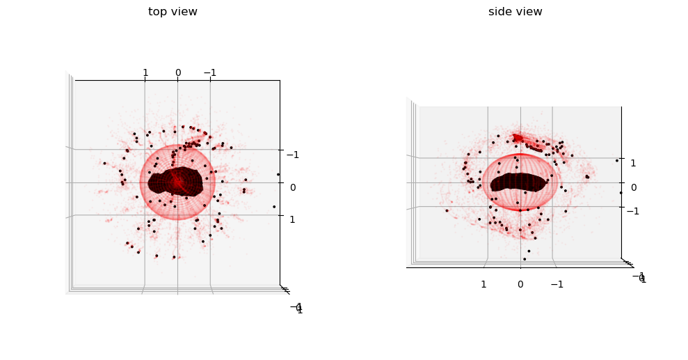
Note
The collision avoidance manouvres appear clusered in specific areas defined by the complex dynamics. If present, all manouvres to keep the swarm within the defined range happen, as expected, at the surface of the spheres defining the allowed zone.
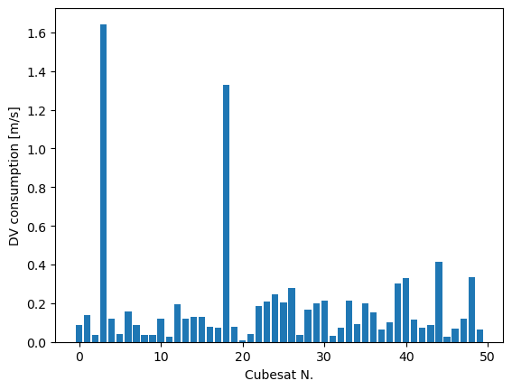
We also plot the \(DV\) distribution.
fig = plt.figure()
plt.bar(range(n_cubesats), DV)
plt.xlabel("Cubesat N.")
plt.ylabel("DV consumption [m/s]")
Text(0, 0.5, 'DV consumption [m/s]')
That is all folks! Pretty cool stuff if you ask me.