Conjunctions#

In this tutorial we consider the simulation we described in quickstart, but instead of stopping at a collision, to then have the possibility to react and proceed, we will only track conjunctions and switch off collisions.

Let us start with some imports:

# core imports
import cascade as csc
import pykep as pk
import numpy as np
import heyoka as hy

# plotting
from mpl_toolkits.mplot3d import Axes3D
from matplotlib import pyplot as plt
%matplotlib inline

The dynamics#

For this tutorial we will make use the same non dimensional Keplerian dynamics used in quickstart.

Let us instantiate it:

dyn = csc.dynamics.kepler(mu = 1)

The initial conditions#

As initial conditions we also repeat the same as in quickstart.

N = 1000 # number of objects simulated
# The following numpy array will hold all the initial conditions and object radius [x,y,z,vx,vy,vz,r]
ic_state = np.zeros((N, 7))
# We generate randomly orbital parameters and imensions and transform them to Cartesian state. Note we make use of nondimensional units as defined in the dynamics.
for i in range(N):
    a = np.random.uniform(1.02, 1.3)
    e = np.random.uniform(0, 0.02)
    inc = np.random.uniform(np.pi/3, np.pi/3 + 0.05)
    om = np.random.uniform(0, 2*np.pi)
    Om = np.random.uniform(np.pi/3, np.pi/3 + 0.05)
    nu = np.random.uniform(0, 2*np.pi)
    size = np.random.uniform(1e-3/2, 1e-4)
    r, v = pk.par2ic([a, e, inc, Om, om, nu], mu = 1.)
    ic_state[i][:3] = r
    ic_state[i][3:6] = v
    ic_state[i][6] = size

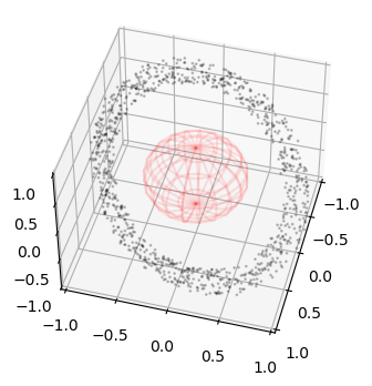
… and we visualize them in proportion to a central body of radius 0.5

fig = plt.figure(figsize=(4,4))
ax = fig.add_subplot(111, projection='3d')

r = 0.5
u, v = np.mgrid[0:2*np.pi:20j, 0:np.pi:10j]
x = r*np.cos(u)*np.sin(v)
y = r*np.sin(u)*np.sin(v)
z = r*np.cos(v)
ax.plot_wireframe(x, y, z, color="r", alpha=0.1)

ax.scatter3D(ic_state[:,0], ic_state[:,1], ic_state[:,2], alpha=0.2, s= 1, c='k')

ax.set_xlim(-1,1)
ax.set_ylim(-1,1)
ax.set_zlim(-1,1)

ax.view_init(45,15)

../_images/b649335c9ca414283e01afc4ee56c81cde8cec53534acf3794a8fdf47ea2f148.png

Building the simulation#

Since we want to track conjunctions and ignore possible collisions, we instantiate the simulation as :

sim = csc.sim(state = ic_state, dyn=dyn, ct = 2*np.pi / 90, conj_thresh = 1e-2, min_coll_radius=float('inf'))

Two arguments have been added with respect to the similar simulation presented in quickstart. The argument conj_thresh defines the conjunction threshold. All conjunction events with closest distance smaller than conj_thresh will be detected and reported. The argument min_coll_radius ignores all collisions between objects having radius smaller than its value. In this case we use infinity hence switching off all collision events.

Running the simulation#

# This will try to propagate all the orbits up to the final time is reached (roughly three orbits)
oc = sim.propagate_until(6 * np.pi)

At the end of this simulation all conjunctions will be stored in the attribute cascade.sim.conjunctions. This contains in each line the idx of the two objects, the conjunction time, the closest distance and the states of the two particles at the conjunction.

conj_n = len(sim.conjunctions)
conj_d = sim.conjunctions['dist']
print("Number of conjunctions: ", len(sim.conjunctions))
print("Minimal conjunction distance: ", min(conj_d))

Number of conjunctions:  473
Minimal conjunction distance:  0.00044759696356493084

Plotting the conjunction positions#

fig = plt.figure(figsize=(4,4))
ax = fig.add_subplot(111, projection='3d')

r = 0.5
u, v = np.mgrid[0:2*np.pi:20j, 0:np.pi:10j]
x = r*np.cos(u)*np.sin(v)
y = r*np.sin(u)*np.sin(v)
z = r*np.cos(v)
ax.plot_wireframe(x, y, z, color="r", alpha=0.1)

ax.scatter3D(ic_state[:,0], ic_state[:,1], ic_state[:,2], alpha=0.2, s= 1, c='k')

pos = np.array([sim.conjunctions[i][4][:3] for i in range(conj_n)])
ax.scatter3D(pos[:,0], pos[:,1], pos[:,2], alpha=1, s= 3, c='r')

ax.set_xlim(-1,1)
ax.set_ylim(-1,1)
ax.set_zlim(-1,1)

ax.view_init(45,15)

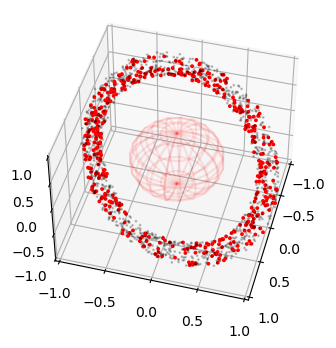
../_images/ad00e04d5edf04c300e5018e64dfd4e9fccc6cab73f4f7c4aacf3cc690ffda12.png

as expected, in this case, conjunctions happen more or less uniformly in the Keplerian ring defined by the orbits.

Conjunctions

Contents