Approximating the hypervolume
Determining the hypervolume indicator is a computationally expensive task. Even in case of a reasonably small dimension and low number of points (e.g. 100 points in 10 dimensions), there are currently no known algorithms that can yield the results fast enough for most multiple-objective optimizers.
In this tutorial we will show a way to compute the hypervolume indicator faster, but at the cost of accuracy. Two algorithms found in PyGMO.util.hv_algorithm are capable of computing the hypervolume approximately:
- PyGMO.util.hv_algorithm.bf_fpras - capable of approximating the hypervolume indicator
- PyGMO.util.hv_algorithm.bf_approx - capable of approximating the least and the greatest contributor
Note
PyGMO.util.hypervolume object will never delegate the computation to any of the approximated algorithms. The only way to use the approximated algorithms is through the explicit request (see the beginning of the tutorial Advanced hypervolume computation and analysis for more information on how to do that).
FPRAS
Algorithm PyGMO.util.hv_algorithm.bf_fpras found in PyGMO is a Fully Polynomial-Time Randomized Approximation Scheme accustomed for the computation of the hypervolume indicator. You can invoke the FPRAS by creating an instance of the hv_algorithm:
from PyGMO import *
from PyGMO.util import *
prob = problem.dtlz(prob_id = 3, fdim=10)
pop = population(prob, 100)
fpras = hv_algorithm.bf_fpras(eps=0.1, delta=0.1)
hv = hypervolume(pop)
ref = hv.get_nadir_point(1.0)
hv.compute(ref, algorithm=fpras)  # Will compute the approximated hypervolume
To influence the accuracy of the FPRAS, it is possible to provide the following keyword arguments to its constructor:
- eps - relative accuracy of the approximation
- delta - probability of error
For given parameters eps=eps0 and delta=delta0, the obtained solution is (with probability 1 - delta0) within a factor of 1 +/- eps0 from the exact hypervolume.
Note
The smaller the eps and delta, the longer it will take for the algorithm to evaluate.
By the relative error, we mean the scenario in which the approximation is accurate within given order of magnitude, e.g. 312.32 and 313.41, are accurate within eps = 0.1, because they are accurate within two orders of magnitude. At the same time, these are NOT accurate within eps = 0.01.
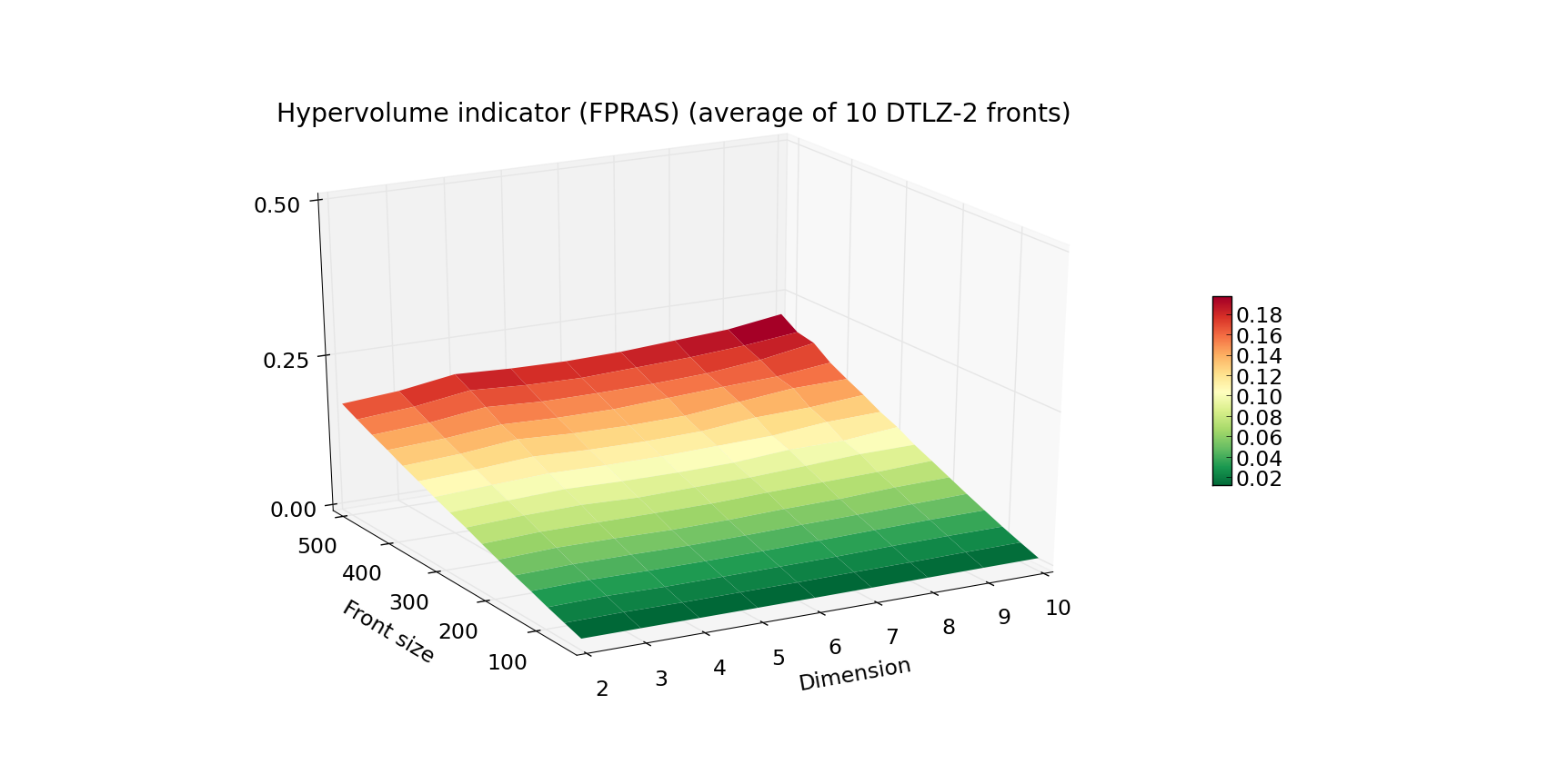
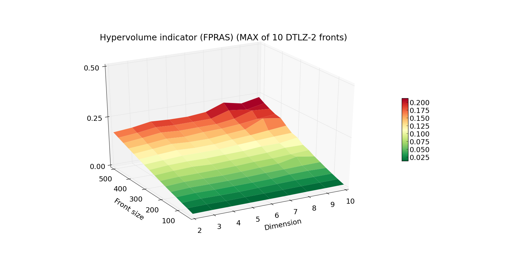
Running time
Plot below presents the measured running time (average and MAX out of 10) of FPRAS for varying Front size and Dimension. The algorithm was instantiated with eps=0.1 and delta=0.1. Notice the lack of any exponential increase in time as the dimension increases.
Since FPRAS scales so well with the dimension size, let us present a more extreme example of fronts for which we again will measure the execution time:
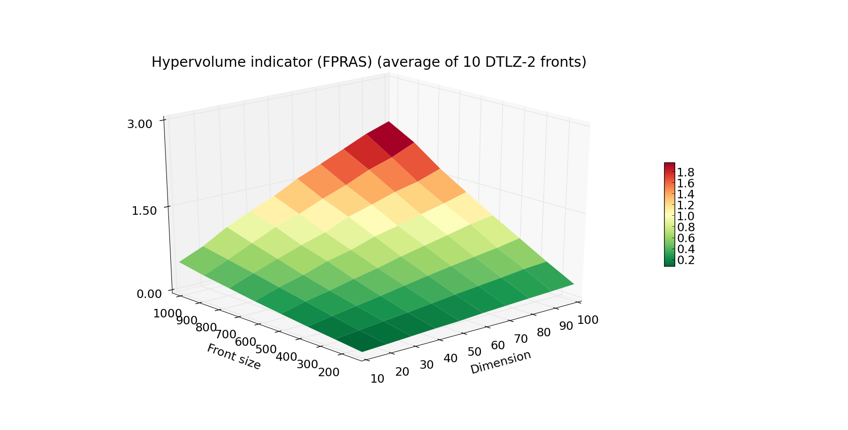
Now, that is quite a feat! A front of 1000 points in 100 dimensions is beyond the reach of the algorithms that rely on the exact computation.
Approximation of the least contributor
Additionally to FPRAS, PyGMO provides an approximated algorithm dedicated for the computation of the least/greatest contributor. This is useful when we want to utilize evolutionary algorithms which rely on that feature, especially when the problems has many objectives.
from PyGMO import *
from PyGMO.util import *
# Problem with 30 objectives and 300 individuals
prob = problem.dtlz(prob_id = 3, fdim=30)
pop = population(prob, 300)

alg = hv_algorithm.bf_approx(eps=0.1, delta=0.1)
hv = hypervolume(pop)
ref = hv.get_nadir_point(1.0)
hv.least_contributor(ref, algorithm=alg)  # Will compute the approximated least contributor
Note
Algorithm bf_approx provides only two features - computation of the least and the greatest contributor. Request for the computation of any other measure will raise and exception.