Covariance Propagation#
In this notebook, we discuss how to use dsgp4 to apply the first order approximation for propagating a covariance matrix:
where \(\textrm{TLE}_0\) is the initial TLE, at time \(t_0\), and \(\pmb{x}\) is the state vector in Cartesian TEME, at a certain propagation time \(t_f\).
Note
An important aspect to notice is that the above formula, besides propagating the covariance, it also transforms the propagated covariance from TLE parameters, to Cartesian ones.
First, let’s do the usual imports:
import dsgp4
import torch
import numpy as np
torch.set_default_dtype(torch.float32)
And let’s also construct some TLE objects:
inp_file='''0 PSLV DEB *
1 35351U 01049QK  22066.70636923  .00002156  00000-0  63479-3 0  9999
2 35351  98.8179  29.5651 0005211  45.5944 314.5671 14.44732274457505
0 COSMOS 2251 DEB
1 34550U 93036UL  22068.48847750  .00005213  00000-0  16483-2 0  9994
2 34550  73.9920 106.8624 0177754 242.5189 115.7794 14.31752709674389
0 GGSE 3
1  1292U 65016C   22069.19982496  .00000050  00000-0  68899-4 0  9998
2  1292  70.0769  62.6868 0022019 223.3241 136.6137 14.00692829906555
0 CZ-2D DEB
1 35275U 08056E   22068.48794021  .00000595  00000-0  24349-3 0  9998
2 35275  98.8424  84.5826 0139050 155.2017 205.5930 14.25810852685662
0 FENGYUN 1C DEB
1 35237U 99025DQV 22069.17158141  .00009246  00000-0  14994-2 0  9992
2 35237  99.5946 147.0483 0055559  41.0775 319.4589 14.70446744775205
'''
tles=inp_file.splitlines()
#propagation times:
tsinces=torch.linspace(0,0.5*60*24,8)#0.5 days propagation
#we construct the TLE batch:
indexes=[]
for i in range(len(tsinces)):
    for k in range(0,len(tles),3):
        indexes.append(tles[k:3+k])
tles=[dsgp4.tle.TLE(index[:3]) for index in indexes]
#let's also repeat the times now:
tsinces=tsinces.repeat(5)
We initialize & propagate the TLEs and track the gradients:
#we initialize the TLEs w gradients:
tle_elements,tle_batch=dsgp4.initialize_tle(tles,with_grad=True)
#propagate the orbits:
state_teme=dsgp4.propagate_batch(tle_batch,tsinces)
Let’s construct the partials of the output w.r.t. the TLE parameters
#now we can build the partial derivatives matrix, of shape Nx6x9 (N is the number of tsince elements, 6 is the number of elements in the state vector, and 9 is the number of elements in the TLE):
dx_dtle = torch.zeros((len(tsinces),6,9))
for k in range(len(tsinces)):
    for i in range(6):
        tle_elements[k].grad=None
        state_teme[k].flatten()[i].backward(retain_graph=True)
        dx_dtle[k,i,:] = tle_elements[k].grad
Now, let’s define some useful parameters:
Cov_xyz=np.zeros((len(tles),6,6))
Cov_rtn=np.zeros((len(tles),6,6))
#this is the initial TLE covariance matrix:
Cov_tle=np.array([[ 1.06817079e-23,  8.85804989e-25,  1.51328946e-24,
        -2.48167092e-13,  1.80784129e-11, -9.17516946e-17,
        -1.80719145e-11,  2.47782854e-14,  1.06374440e-19],
       [ 1.10888880e-26,  9.19571327e-28,  1.57097512e-27,
        -2.57618033e-16,  1.87675528e-14, -9.28440729e-20,
        -1.87608028e-14,  2.57219640e-17,  1.10539220e-22],
       [-3.62208982e-24, -3.00370060e-25, -5.13145502e-25,
         8.41515501e-14, -6.13025898e-12,  3.11161104e-17,
         6.12805538e-12, -8.40212641e-15, -3.61913778e-20],
       [-2.72347076e-13, -2.25849762e-14, -3.85837006e-14,
         6.69613552e-03, -4.60858400e-01,  2.44529381e-06,
         4.60848714e-01, -6.66633934e-04,  2.73554382e-10],
       [ 1.98398791e-11,  1.64526723e-12,  2.81073778e-12,
        -4.60858400e-01,  3.35783115e+01, -1.70385711e-04,
        -3.35662070e+01,  4.60149046e-02,  1.68286334e-07],
       [-1.00692291e-16, -8.34937429e-18, -1.42650203e-17,
         2.44529381e-06, -1.70385711e-04,  1.75093676e-05,
         1.70379140e-04, -2.42796071e-07, -2.62336921e-10],
       [-1.98327475e-11, -1.64467582e-12, -2.80972744e-12,
         4.60848714e-01, -3.35662070e+01,  1.70379140e-04,
         3.35541747e+01, -4.60131157e-02, -2.28248504e-07],
       [ 2.71925407e-14,  2.25500097e-15,  3.85239630e-15,
        -6.66633934e-04,  4.60149046e-02, -2.42796071e-07,
        -4.60131157e-02,  6.63783423e-05, -3.21657063e-12],
       [ 1.16764843e-19,  9.73507662e-21,  1.65971417e-20,
         2.73554368e-10,  1.68286335e-07, -2.62336921e-10,
        -2.28248505e-07, -3.21656925e-12,  2.21029182e-07]])/1000.
frob_norms=np.zeros((len(tles),))

def rotation_matrix(state):
    """
    Computes the UVW rotation matrix.

    Args:
        state (`numpy.array`): numpy array of 2 rows and 3 columns, where
                                    the first row represents position, and the second velocity.

    Returns:
        `numpy.array`: numpy array of the rotation matrix from the cartesian state.
    """
    r, v = state[0], state[1]
    u = r / np.linalg.norm(r)
    w = np.cross(r, v)
    w = w / np.linalg.norm(w)
    v = np.cross(w, u)
    return np.vstack((u, v, w))

def from_cartesian_to_rtn(state, cartesian_to_rtn_rotation_matrix=None):
    """
    Converts a cartesian state to the RTN frame.

    Args:
        state (`numpy.array`): numpy array of 2 rows and 3 columns, where
                                    the first row represents position, and the second velocity.
        cartesian_to_rtn_rotation_matrix (`numpy.array`): numpy array of the rotation matrix from the cartesian state. If None, it is computed.

    Returns:
        `numpy.array`: numpy array of the RTN state.
    """
    # Use the supplied rotation matrix if available, otherwise compute it
    if cartesian_to_rtn_rotation_matrix is None:
        cartesian_to_rtn_rotation_matrix = rotation_matrix(state)
    r, v = state[0], state[1]
    r_rtn = np.dot(cartesian_to_rtn_rotation_matrix, r)
    v_rtn = np.dot(cartesian_to_rtn_rotation_matrix, v)
    return np.stack([r_rtn, v_rtn]), cartesian_to_rtn_rotation_matrix
Finally, we can propagate all covariances…
for idx, tle in enumerate(tles):
    state_rtn, cartesian_to_rtn_rotation_matrix = from_cartesian_to_rtn(state_teme[idx].detach().numpy())
    #I construct the 6x6 rotation matrix from cartesian -> RTN
    transformation_matrix_cartesian_to_rtn = np.zeros((6,6))
    transformation_matrix_cartesian_to_rtn[0:3, 0:3] = cartesian_to_rtn_rotation_matrix
    transformation_matrix_cartesian_to_rtn[3:,3:] = cartesian_to_rtn_rotation_matrix

    Cov_xyz[idx,:,:]=np.matmul(np.matmul(dx_dtle[idx,:],Cov_tle),dx_dtle[idx,:].T)
    frob_norms[idx]=np.linalg.norm(Cov_xyz[idx,:,:],ord='fro')
    Cov_rtn[idx,:,:]=np.matmul(np.matmul(transformation_matrix_cartesian_to_rtn, Cov_xyz[idx,:,:]),transformation_matrix_cartesian_to_rtn.T)
/var/folders/vf/cj60m8k162316snsvmjw65280000gp/T/ipykernel_16046/2216534334.py:8: DeprecationWarning: __array_wrap__ must accept context and return_scalar arguments (positionally) in the future. (Deprecated NumPy 2.0)
  Cov_xyz[idx,:,:]=np.matmul(np.matmul(dx_dtle[idx,:],Cov_tle),dx_dtle[idx,:].T)
/var/folders/vf/cj60m8k162316snsvmjw65280000gp/T/ipykernel_16046/2216534334.py:8: DeprecationWarning: __array__ implementation doesn't accept a copy keyword, so passing copy=False failed. __array__ must implement 'dtype' and 'copy' keyword arguments.
  Cov_xyz[idx,:,:]=np.matmul(np.matmul(dx_dtle[idx,:],Cov_tle),dx_dtle[idx,:].T)
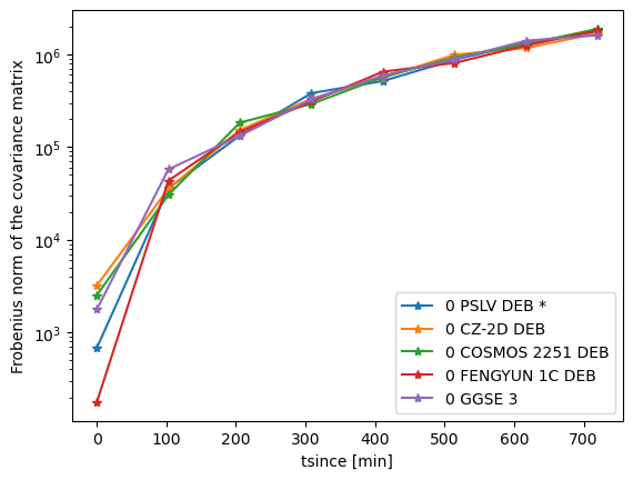
Let’s plot the Frobenius norm of each covariance for each TLE, as a function of time from TLE:
import matplotlib.pyplot as plt

indexes=[0,8,16,24,32,40]
for i in range(len(indexes)-1):
    plt.semilogy(tsinces[indexes[i]:indexes[i+1]].detach().numpy(),frob_norms[indexes[i]:indexes[i+1]],'-*',label=tles[indexes[i]].line0)
plt.legend()
plt.xlabel('tsince [min]')
plt.ylabel('Frobenius norm of the covariance matrix')
Text(0, 0.5, 'Frobenius norm of the covariance matrix')