Designing and optimizing interplanetary trajectories

PyGMO can be used to optimize spacecraft trajectories by using the MGA-1DSM problem. An instance of this problem contains the sequence of planets, you want to visit with your spacecraft as well as its launch window, its starting velocity and bounds for the time of flight. Between each planetary encounters, a deep space manouver can be performed. The objective is to lower the total Delta-V spend for the travel, as this corresponds directly to the mass of fuel needed.

NOTE: Even though this example will work with PyGMO, you need to install PyKEP in order to use other values than the default.

Lets launch PyGMO and start by creating the default problem:

ipython --pylab

from PyGMO import *
alg = algorithm.jde(memory=True)
prob = problem.mga_1dsm_tof()

By default the sequence is Earth - Venus - Earth, so there are two “legs” (1. Earth to Venus and 2. Venus to Earth) to optimize at the same time. By default we give a minimum of 50 and a maximum of 900 days to each leg. If you don’t believe this, check for yourself:

prob.get_sequence()
prob.get_tof()

There are also default values for the other parameters, but you don’t have to worry about those details. This version of the problem mga_1dsm_tof (see: PyGMO.problem.mga_1dsm_tof) is particularly useful if you know some bounds on the travel time for your legs. If you have no clue though, you can use the problem mga_1dsm_alpha (see: PyGMO.problem.mga_1dsm_alpha) instead where you can specify just the bounds for the overall time of flight with the tof keyword. The alpha-version is also particularly useful for multi-objective optimization. By using the multi_objective keyword as an argument you can instantiate the problem with two objectives (Delta-V and total time of flight) instead of just one (Delta-V).

# initialize the trajectory problem to design a tour within 1 to 5 years
prob_alpha = problem.mga_1dsm_alpha(tof=[1 * 365.25, 5 * 365.25], multi_objective=True)

For the remainder of this example, lets return to the original single-objective problem and start some optimizations runs:

l = list()
for i in range(30):
    archi = archipelago(alg,prob,8,10,topology = topology.fully_connected())
    for j in range(30):
        archi.evolve(5)
        print min([isl.population.champion.f[0] for isl in archi])
    tmp = [isl for isl in archi]; tmp.sort(key = lambda x: x.population.champion.f[0]);
    l.append(tmp[0].population.champion)
print "Results: \n"
print [ch.f[0] for ch in l]

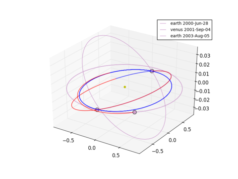
We may then plot the trajectory and look at some additional informations:

# sort list and extract chromosome of the solution of lowest Delta-V
l.sort(key = lambda x: x.f[0])
x_so = l[0].x
prob.plot(x_so)
print prob.pretty(x_so)

That looks nice! Now we are interested in a trade-off between the Delta-V and the the total time of travel. We will use this solution (x_so) of a low Delta-V and inject it into a new population. This will help when we optimize the population by a multi-objective optimizer for low Delta-V and short time of travel at the same time, building up an approximation of the Pareto-front. For this, we reinitialize the problem to be multi-objective and change the algorithm.

alg = algorithm.nsga_II()
prob = problem.mga_1dsm_tof(multi_objective=True)

We will use the island model to improve the overall optimization. Each island works just on a small fraction of solutions and is thus faster as when operating on a single large population.

sel = migration.best_s_policy(10)
rep = migration.fair_r_policy(10)
archi = archipelago(topology = topology.fully_connected())
pop = population(prob,39)
# we inject the solution of the single-objective optimization here to get a population of 100
pop.push_back(x_so)
isl = island(alg,pop,s_policy=sel, r_policy=rep)
archi.push_back(isl)
# we fill up the archipelago with 9 other island initialized by random without injection
for i in range(9):
    archi.push_back(island(alg,prob,40,s_policy=sel, r_policy=rep))
archi.evolve(40)
archi.join()

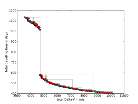
The injected solution will spread by migration to all other islands in the archipelago. After enough generations, all islands should have converged to similar fronts. Lets put them all together in a single population and have a look at the Pareto-front:

pop = population(prob)
for isl in archi:
    for ind in isl.population:
        pop.push_back(ind.cur_x)
pop.plot_pareto_fronts()
# highlight the solutions of the 1st island with red
archi[0].population.plot_pareto_fronts(rgb=(1,0,0))
ylabel('total travelling time in days')
xlabel('total Delta-V in m/s')

You see a discontinuity in this picture which is very interesting: It allows you to save over a year of travelling time by just using a bit more Delta-V around 4709 m/s.