Plotting

In this tutorial we will explore the basic plotting tools provided by pykep via its plot module. The module was built as to facilitate the incremental construction of plots showing trajectories and other important quantities of interest when planning/designing interplanetary missions.

We start importing the basics:

import pykep as pk
import numpy as np

%matplotlib inline

3D Plots

Plot planets

In most cases one would want to start creating a 3D empty canvas where to incrementally add details. To do so we can avoid a direct interaction with the backend matplotlib using the convenience make_3Daxis factory:

ax = pk.plot.make_3Daxis(figsize = (3,3));

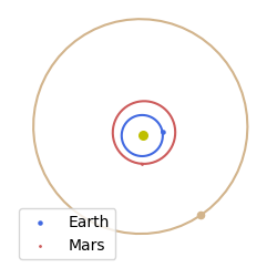
We may then add the Sun and a few planets easily … in the code below we will make use of the JPL low precision ephemerides, and thus use the jpl_lp User Defined Planet, but any other udpla would work.

# Earth
udpla = pk.udpla.jpl_lp(body="EARTH")
earth = pk.planet(udpla)

# Mars
udpla = pk.udpla.jpl_lp(body="MARS")
mars = pk.planet(udpla)

#Jupiter
udpla = pk.udpla.jpl_lp(body="JUPITER")
jupiter = pk.planet(udpla)

# Plotting (both the orbit and the planet)
ax = pk.plot.make_3Daxis(figsize = (3,3))
pk.plot.add_sun(ax)

pk.plot.add_planet_orbit(ax, earth, plot_range = [0, 365.25], c = "royalblue", label = "")
pk.plot.add_planet(ax, earth, when = 0, c = "royalblue", s = 5, label="Earth")

pk.plot.add_planet_orbit(ax, mars, label = "", c = "indianred")
pk.plot.add_planet(ax, mars, when = 0, c = "indianred", s = 1, label = "Mars")

pk.plot.add_planet_orbit(ax, jupiter, label = "", c = "tan")
pk.plot.add_planet(ax, jupiter, when = 0, c = "tan")

ax.legend()
ax.set_xlim3d(-4,4)
ax.set_ylim3d(-4,4)
ax.axis('off')
ax.view_init(90,0)

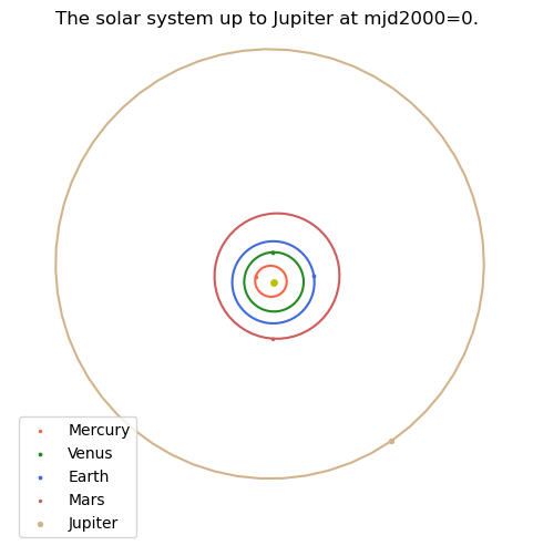
In some cases it may be useful to add solar system planets at once to a plot. The add_solar_system does just that:

ax = pk.plot.make_3Daxis(figsize = (6,6))
ep = pk.epoch(0)
pk.plot.add_solar_system(ax, bodies = [1,2,3,4,5], when = ep)
ax.view_init(90,0)
ax.legend()
ax.axis('off')
ax.set_xlim3d(-4,4)
ax.set_ylim3d(-4,4)
ax.view_init(90,0)
ax.set_title("The solar system up to Jupiter at mjd2000=0.");

Plot a Lambert arc

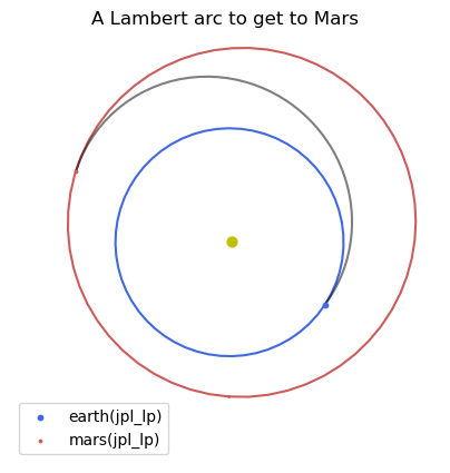
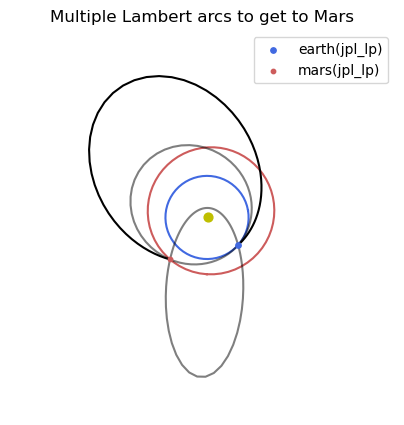
The class lambert_problem is used to compute all ballistic arcs transfering in a fixed time of flight from a starting to a final position. In general there are more solutions for a given geometry, in pykep the user can plot all of them easily. Lets see how. First we create a Lambert problem, say an Earth-Mars transfer.

t0 = 4340.
tof_days = 280.22
r0, v0 = earth.eph(t0)
r1, v1 = mars.eph(t0+tof_days)
lp = pk.lambert_problem(r0=r0, r1=r1,mu=pk.MU_SUN, tof=tof_days*pk.DAY2SEC )

We can now assemble a plot

# Making the axis
ax = pk.plot.make_3Daxis(figsize = (5,5))

# Adding the various planets / Sun
pk.plot.add_sun(ax, s=40)

pk.plot.add_planet(ax, earth, when=t0, label = earth.get_name(), c = 'royalblue', s=10)
pk.plot.add_planet_orbit(ax, earth, c = 'royalblue')

pk.plot.add_planet(ax, mars, when=t0 + tof_days, label = mars.get_name(), c = 'indianred', s=3)
pk.plot.add_planet_orbit(ax, mars, c = 'indianred')

# Here we add the Lambert arc
pk.plot.add_lambert(ax, lp, N=60, sol=0, c='k', alpha=0.5)

# Some cosmetics to customize the plot
ax.legend()
ax.axis('off')
ax.set_xlim3d(-1.2,1.2)
ax.set_ylim3d(-1.2,1.2)
ax.view_init(90,0)
ax.set_title("A Lambert arc to get to Mars");

t0 = 2140.
tof_days = 1230.22
r0, v0 = earth.eph(t0)
r1, v1 = mars.eph(t0+tof_days)
lp = pk.lambert_problem(r0=r0, r1=r1,mu=pk.MU_SUN, tof=tof_days*pk.DAY2SEC)

# Making the axis
ax = pk.plot.make_3Daxis(figsize = (5,5))

# Adding the various planets / Sun
pk.plot.add_sun(ax, s=40)

pk.plot.add_planet(ax, earth, when=t0, label = earth.get_name(), c = 'royalblue', s=15)
pk.plot.add_planet_orbit(ax, earth, c = 'royalblue')

pk.plot.add_planet(ax, mars, when=t0 + tof_days, label = mars.get_name(), c = 'indianred', s=10)
pk.plot.add_planet_orbit(ax, mars, c = 'indianred')

# Here we add the Lambert arc
pk.plot.add_lambert(ax, lp, N=60, sol=0, c='k', alpha=1.)
pk.plot.add_lambert(ax, lp, N=60, sol=1, c='k', alpha=0.5)
pk.plot.add_lambert(ax, lp, N=120, sol=2, c='k', alpha=0.5)



# Some cosmetics to customize the plot
ax.legend()
ax.axis('off')
ax.set_xlim3d(-3,3)
ax.set_ylim3d(-3,3)
ax.view_init(90,0)
ax.set_title("Multiple Lambert arcs to get to Mars");

Plot a Sims-Flanagan trajectory leg.

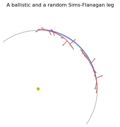
The class sims_flanagan is used to represent a low-thrust interplanetary trajectory of a spacecraft, modelled using a sequence of impulsive \(\Delta V\). We can visualize, using the plot module, this trajectory and inspect visually the underlying discretization. Clarly the trajectory will only close if the throttle sequence (the low-thrust strategy) results in a feasible trajectory.

Lets start to instantiate a Sims-Flanagan leg, the default constructor will construct a feasible non-dimensional ballistic transfer (with a rather big maximum thrust):

sf = pk.leg.sims_flanagan()
nseg = 20
sf.throttles=[0,0,0] * nseg

which we can immediately visualize, together with a random variation produced by randomly initializing the throttle history:

# Making the axis
ax = pk.plot.make_3Daxis(figsize = (5,5))

# Adding the Sun and the Earth for added coolness and reference.
pk.plot.add_sun(ax, s=40)
pk.plot.add_planet_orbit(ax, earth, c = 'black', alpha=0.3)

# And plotting the leg (ballistic)
pk.plot.add_sf_leg(ax, sf, units=1., show_throttles=True, length=0.1, arrow_length_ratio=0.2)

# And plotting the leg (random thrust)
sf.throttles = 1 - 2*np.random.random((nseg*3, ))
pk.plot.add_sf_leg(ax, sf, units=1., show_throttles=True, length=0.1, arrow_length_ratio=0.2)

ax.view_init(90,270)
ax.set_xlim3d(-0.2,1)
ax.set_ylim3d(-0.2,1)
ax.axis('off')

ax.set_title("A ballistic and a random Sims-Flanagan leg");