Low-thrust transfers via indirect methods I (mass-fixed time)

In this notebook we show how to solve the minimum mass Optimal Control Problem (OCP) for a fixed time low-thrust interplanetary transfer employing an indirect method.

Indirect methods are follow rather mechanic developments: starting from the dynamics a TPBVP (Two-Point-Boundary-Value-Problem) is built applying Pontryagin maximum (minimum, in our case) principle. The TPBVP is defined on an augmented ODE system and solved by means of single or multiple shooting methods.

In this notebook we guide, step-by-step, the reader in the application of such a method in a widely encountered case in space flight mechanics, the low-thrust minimum time problem. Eventually use pykep native tools to quickly skip the tedious parts.

import pykep as pk
import numpy as np
import heyoka as hy
import pygmo as pg
import pygmo_plugins_nonfree as ppnf

from matplotlib import pyplot as plt

Manual construction of the TPBVP

We consider the dynamics:

\[\begin{split} \left\{ \begin{array}{l} \dot{\mathbf r} = \mathbf v \\ \dot{\mathbf v} = -\frac{mu}{r^3}\mathbf r + c_1 \frac um \hat{\mathbf i}\\ \dot{m} = - \frac{c_1}{c_2} u \end{array} \right. \end{split}\]

where \(c_1=T_{max}\) is the maximum thrust that the spacecarft propulsion can deliver, while \(c_2 = I_{sp} g_0\).

We also introduce as many auxiliary functions \(\mathbf \lambda\) (the co-states) are there are state variables. Using heyoka as a symbolic manipulator, let us introduce symbols for all the time dependent quantities:

# The state
x, y, z, vx, vy, vz, m = hy.make_vars("x", "y", "z", "vx", "vy", "vz", "m")
# The costate
lx, ly, lz, lvx, lvy, lvz, lm = hy.make_vars(
    "lx", "ly", "lz", "lvx", "lvy", "lvz", "lm"
)
# The controls
u, ix, iy, iz = hy.make_vars("u", "ix", "iy", "iz")

As to write comfortably the various developments, we introduce some useful expressions and regroup some of our variable into 3D vectors:

# Useful expressions
r3 = (x**2 + y**2 + z**2) ** (1.5)
lv_norm = hy.sqrt(lvx**2 + lvy**2 + lvz**2)
rho = 1 - hy.par[1] * lv_norm / m / hy.par[4] - hy.par[1] / hy.par[2] * lm / hy.par[4]

# Vectors for convenience of math manipulation
lr = np.array([lx, ly, lz])
lv = np.array([lvx, lvy, lvz])
r = np.array([x, y, z])
v = np.array([vx, vy, vz])
i_vers = np.array([ix, iy, iz])

Note how the various constants of our problem are considered as heyoka parameters in the following order: \([\mu, c_1, c_2, \epsilon, \lambda_0]\), \(c_1 = T_{max}\), \(c_2 = \frac{T_{max}}{I_{sp}g_0}\)

The dynamics can then be written as:

# Dynamics
fr = v
fv = hy.par[1] * u / m * i_vers - (hy.par[0] / r3) * r
fm = -hy.par[1] / hy.par[2] * u

We introduce the Hamiltonian (\(\mathbf x\) is the whole state, \(\mathbf \lambda\) is the whole co-state, and \(\mathbf u\) represent are all the controls),

\[ \mathcal H(\mathbf x, \mathbf \lambda, \mathbf u) = \mathbf \lambda_r \cdot \mathbf f_r + \mathbf \lambda_v \cdot \mathbf f_v + \lambda_m f_m + \lambda_0 \left(u + \epsilon\log(u(1-u))\right) \]

# Hamiltonian
H_full = lr @ fr + lv @ fv + lm * fm + hy.par[4] * (u - hy.par[3] * hy.log(u * (1 - u)))

And write the resulting Hamiltonian system:

\[\begin{split} \left\{ \begin{array}{l} \dot{\mathbf x} = \frac{\partial \mathcal H}{\partial \mathbf \lambda} \\ \dot{\mathbf \lambda} = - \frac{\partial \mathcal H}{\partial \mathbf x} \\ \end{array}\right. \end{split}\]

# Augmented equations of motion
rhs = [
    hy.diff(H_full, var)
    for var in [lx, ly, lz, lvx, lvy, lvz, lm, x, y, z, vx, vy, vz, m]
]
for j in range(7, 14):
    rhs[j] = -rhs[j]

The minimum principle from Pontryagin requires to find the mimimum in the admissible control space of the Hamiltonian:

\[ \mathbf u^* = \argmin_{\mathbf u \in \mathcal U} \mathcal H(\mathbf x, \mathbf \lambda, \mathbf u) \]

which, in our case, results in:

# We apply Pontryagin minimum principle (primer vector and u^* = 2eps / (rho + 2eps + sqrt(rho^2+4*eps^2)))
argmin_H_full = {
    ix: -lvx / lv_norm,
    iy: -lvy / lv_norm,
    iz: -lvz / lv_norm,
    u: 2
    * hy.par[3]
    / (rho + 2 * hy.par[3] + hy.sqrt(rho * rho + 4 * hy.par[3] * hy.par[3])),
}

Thanks to the above relations, the control is now a continuous differentiable function of the states and costates and thus the dynamics as well as the Hamiltonian can be reworked:

rhs = hy.subs(rhs, argmin_H_full)

# We also build the Hamiltonian as a function of the state / co-state only
# (i.e. no longer of controls now solved thanks to the minimum principle)
H = hy.subs(H_full, argmin_H_full)

The following code block thus instantiate the heyoka integrator as well as other convenience functions.

# We compile the Hamiltonian into a C function (to be called with pars = [mu, c1, c2, eps, l0])
H_func = hy.cfunc([H], [x, y, z, vx, vy, vz, m, lx, ly, lz, lvx, lvy, lvz, lm])
# We compile the thrust direction
u_func = hy.cfunc(
    [argmin_H_full[u]], [x, y, z, vx, vy, vz, m, lx, ly, lz, lvx, lvy, lvz, lm]
)
# We compile the SF
rho_func = hy.cfunc([rho], [x, y, z, vx, vy, vz, m, lx, ly, lz, lvx, lvy, lvz, lm])
# We compile also the thrust direction
i_vers_func = hy.cfunc(
    [argmin_H_full[ix], argmin_H_full[iy], argmin_H_full[iz]], [lvx, lvy, lvz]
)
# We assemble the Taylor adaptive integrator
full_state = [x, y, z, vx, vy, vz, m, lx, ly, lz, lvx, lvy, lvz, lm]
sys = [(var, dvar) for var, dvar in zip(full_state, rhs)]
ta = hy.taylor_adaptive(sys, state=[1.0] * 14)

Constructing the TPBVP using pykep

For the specific case outlined above pykep offers a convenient series of pre-assembled functions and objects which basically construct the same objects as above. These can turn out to be useful for analysis of specific cases, but in general they are used internally by the various UDP provided in pykep hence the user in most cases does not need to care.

# The Taylor integrator
ta = pk.ta.get_pc(1e-16, pk.optimality_type.MASS)
# The Variational Taylor integrator
ta = pk.ta.get_pc_var(1e-16, pk.optimality_type.MASS)
# The Hamiltonian
H_func = pk.ta.get_pc_H_cfunc(pk.optimality_type.MASS)
# The switching function
SF_func = pk.ta.get_pc_SF_cfunc(pk.optimality_type.MASS)
# The magnitude of the throttle
u_func = pk.ta.get_pc_u_cfunc(pk.optimality_type.MASS)
# The thrust direction
i_vers_func = pk.ta.get_pc_i_vers_cfunc(pk.optimality_type.MASS)
# The dynamics cfunc
dyn_func = pk.ta.get_pc_dyn_cfunc(pk.optimality_type.MASS)

Solving in single shooting

All the code above was merely used for explanatory purposes. Now we scratch all of that and use the dedicated pykep clsses.

We use, as a test case, a simple transfer between two orbits at 1AU. The transfer is simple enough to allow fast convergence and to directly go for a mass optimal trajectory, without using continuation, so that we can directly start using a value \(\epsilon << 1\).

Later, we will also study a case where we need a continuation technique to bring \(\epsilon\) to low values.

# Testcase 1 (easy, no homotopy)
posvel0 = [
    [34110913367.783306, -139910016918.87585, -14037825669.025244],
    [29090.9902134693, 10000.390168313803, 1003.3858682643288],
]
posvelf = [
    [-159018773159.22266, -18832495968.945133, 15781467087.350443],
    [2781.182556622003, -28898.40730995848, -483.4533989771214],
]
tof = 250
mu = pk.MU_SUN
eps = 1e-5

We instantiate the shooting method using the UDP provided by pykep:

udp = pk.trajopt.pontryagin_cartesian_mass(
    posvel0=posvel0,
    posvelf=posvelf,
    tof=tof,
    mu=mu,
    eps=eps,
    T_max=0.6,
    Isp=3000,
    m0=1500,
    L=pk.AU,
    TIME=pk.YEAR2DAY * pk.DAY2SEC,
    MASS=1500,
    with_gradient=True,
)
prob = pg.problem(udp)
prob.c_tol = 1e-6

To solve this problem, we can use both SPQ methods and interior point methods. In this notebook, we make use of the widely available IPOPT solver, which has the great advantage to be also be fully open-source.

ip = pg.ipopt()
ip.set_numeric_option("tol", 1e-9)  # Change the relative convergence tolerance
ip.set_integer_option("max_iter", 50)  # Change the maximum iterations
ip.set_integer_option("print_level", 0)  # Makes Ipopt unverbose
ip.set_string_option(
    "nlp_scaling_method", "none"
)  # Removes any scaling made in auto mode
ip.set_string_option(
    "mu_strategy", "adaptive"
)  # Alternative is to tune the initial mu value
algo = pg.algorithm(ip)

To solve the problem here we use a multi-start teachnique, since this is in genral a good practice. In this specific case convergence is immediate and multiple starts are not strictly necessary.

masses = []
xs = []
for i in range(30):
    pop = pg.population(prob, 1)
    pop = algo.evolve(pop)
    if prob.feasibility_f(pop.champion_f):
        print(". Success!!", end="")
        udp.fitness(pop.champion_x)
        xs.append(pop.champion_x)
        masses.append(udp.ta.state[6])
        break
    else:
        print("x", end="")
print(f"\nFinal mass is: {masses[0]*udp.MASS}")
print(f"Hamiltonian at the final point is: {H_func(udp.ta.state, pars=udp.ta.pars)} \n")

******************************************************************************
This program contains Ipopt, a library for large-scale nonlinear optimization.
 Ipopt is released as open source code under the Eclipse Public License (EPL).
         For more information visit https://github.com/coin-or/Ipopt
******************************************************************************

. Success!!
Final mass is: 1259.9008822026458
Hamiltonian at the final point is: [-0.84850604] 

Let us visualize what we found ….

ax3D = udp.plot(pop.champion_x)
ax3D.view_init(90, 0)

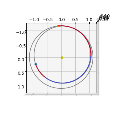
Thrust arcs are indicated with a red color, ballistic with blue.

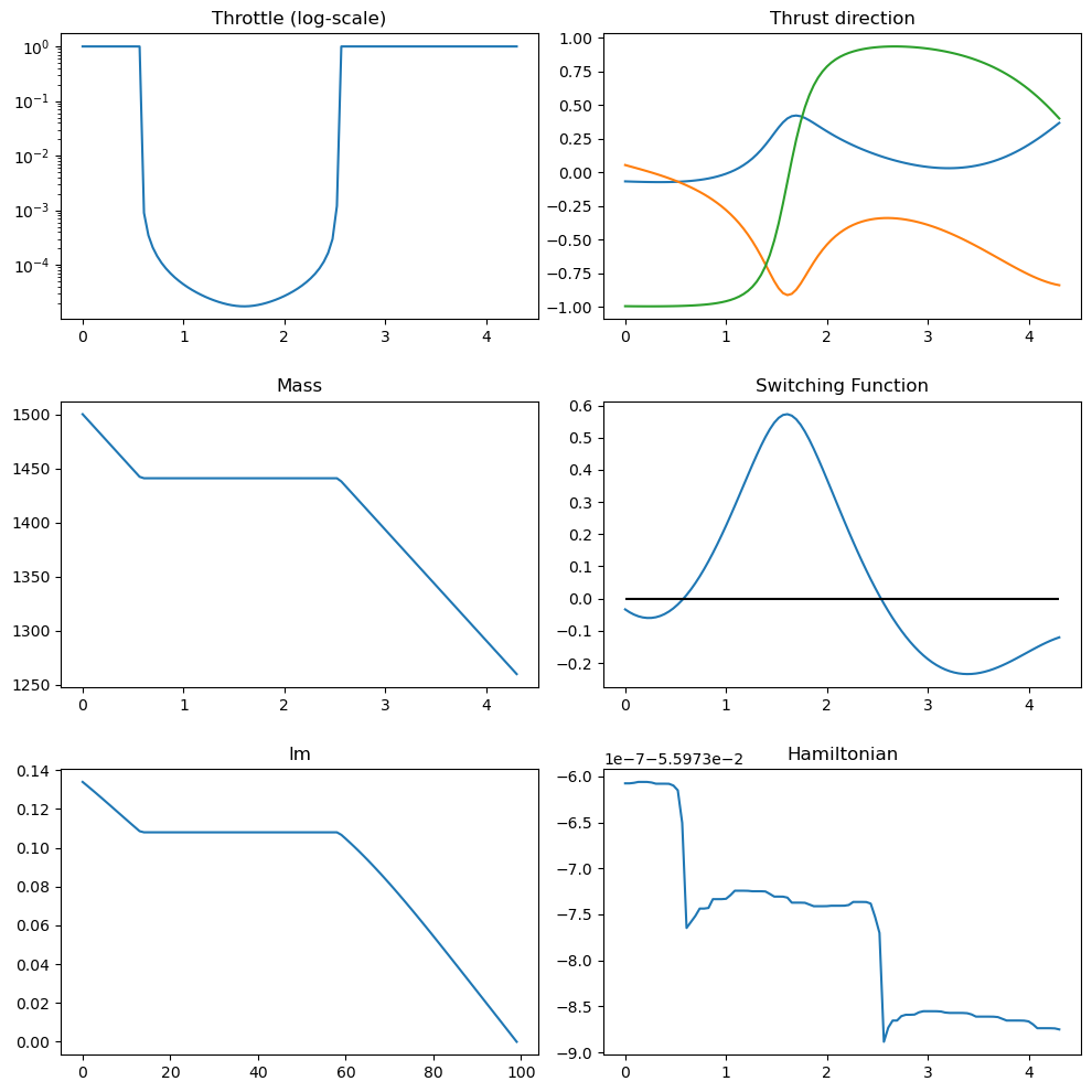
udp.plot_misc(pop.champion_x);

Homotopy

The case above was an easy solve for our single shooting technique. In may cases, especially when multiple revolutions appear or intricate switching functions describe the optimal solution, this will not be the case. In that case homotopy (continuation) methods can help to find a solution.

Here we show how to implement such methods. We use, as test case, a more complex case (coming from an Earth-Mars transfer) where solving directly for mass optimality (e.g. \(\epsilon = 1e-4\) would not work).

The conditions are as follows:

# Testcase 2 (less easy, homotopy needed) [Earth-Mars]
posvel0 = [
    [-125036811000.422, -83670919168.87277, 2610252.8064399767],
    [16081.829029183446, -24868.923007449284, 0.7758272135425942],
]
posvelf = [
    [-169327023332.1986, -161931354587.78766, 763967345.9733696],
    [17656.297796509956, -15438.116653052988, -756.9165272457421],
]
tof = 550. #days
mu = pk.MU_SUN
eps = 1e-1

Exponential homotopy on \(\epsilon\)

Here we decrease the \(\epsilon\) parameter exponentially and use as predictor for the new decision vector corresponding to each successive new value of \(\epsilon\), the previous decision vector. This method forces the step size on the epsilon exponential decrease to small values.

# We instantiate a new optimzation roblem (a pygmo UDP) with the new parameters:
udp = pk.trajopt.pontryagin_cartesian_mass(
    posvel0=posvel0,
    posvelf=posvelf,
    tof=tof,
    mu=mu,
    eps=eps,
    T_max=0.6,
    Isp=3000,
    m0=1500,
    L=pk.AU,
    TIME=pk.YEAR2DAY * pk.DAY2SEC,
    MASS=1500,
    with_gradient=True,
)
prob = pg.problem(udp)
prob.c_tol = 1e-6

The following code block implements an exponential homotopy over \(\epsilon\).

import time
from copy import deepcopy
from IPython.display import clear_output

# No initial guess
first = True
epsilon = 1e-1
decrease_factor = 0.85

# Solve
while True:
    # Set the current epsilon in the udp and construct a problem 
    # (a copy here will be made, so that the udp inside the prob object
    # is a different udp)
    udp.eps = epsilon
    prob = pg.problem(udp)
    prob.c_tol = 1e-6

    # First time looks for a solution, then it continues it
    if first:
        # Creates a random ic population
        pop = pg.population(prob, 1)
        # Starts the time to profile the homotopy time only 
        # (i.e. we exclude the effort to find the first valid traj)
        tstart_tot = time.time()
    else:
        # Use predicted new chromosome
        pop = pg.population(prob)
        pop.push_back(predicted_chromosome)

    # Evolve
    tstart = time.time()
    pop = algo.evolve(pop)
    tend = time.time()

    # Compute constraint violation norm
    err = np.linalg.norm(pop.champion_f[1:])

    # If we find a feasible solution (either the first or a continued one, we log and start the predictor)
    if prob.feasibility_f(pop.champion_f):
        first = False
        clear_output(wait=True)
        print(
            f". Success!! | Error: {err:.2e} | CPU time: {tend-tstart:.2e} | Epsilon = {epsilon:.4e}"
        )

        # Save decision vector for current epsilon (which will be used as an initial guess in the next iteration)
        predicted_chromosome = deepcopy(pop.champion_x)
        best_epsilon = epsilon

        # Save current epsilon (needed if iteration fails)
        epsilon_previous = epsilon

        # Decrease epsilon
        epsilon = epsilon * decrease_factor

        # Stopping condition (desired epsilon reached)
        if epsilon < 1e-4:
            print(
                f"Desired epsilon reached ! | Error: {err:.2e} | CPU time: {tend-tstart:.2e} | Epsilon = {epsilon:.4e}"
            )
            break

    else:
        clear_output(wait=True)
        print(
            f"x | Error: {err:.2e} | CPU time: {tend-tstart:.2e} | Epsilon = {epsilon:.4e}"
        )

        # If first iteration fails, try again with different initial guess
        if first:
            pass

        # Epsilon is too small, we need to increase it (halfway between previous and current)
        else:
            epsilon_previous_new = epsilon
            epsilon = epsilon + abs(epsilon_previous - epsilon) / 2
            epsilon_previous = epsilon_previous_new
tend_tot = time.time()
print(f"Total CPU time: {tend_tot - tstart_tot:.2e}")

. Success!! | Error: 1.99e-11 | CPU time: 1.67e-01 | Epsilon = 1.0854e-04
Desired epsilon reached ! | Error: 1.99e-11 | CPU time: 1.67e-01 | Epsilon = 9.2260e-05
Total CPU time: 3.82e+00

We could obtain a better total computational time if we could just use a higher exponential decrease factor … but we cannot as the initial guess (the predictor used) is poor, so that we are stuck with this (you can try to decrease the decrease_factor and will see how failures in convergence appear and \(\epsilon\) gets to be increased.)

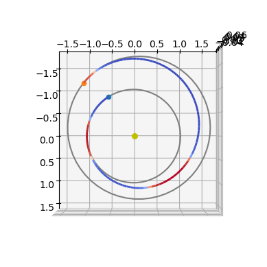
Let us plot what we found …

ax3D = udp.plot(pop.champion_x)
ax3D.view_init(90, 0)

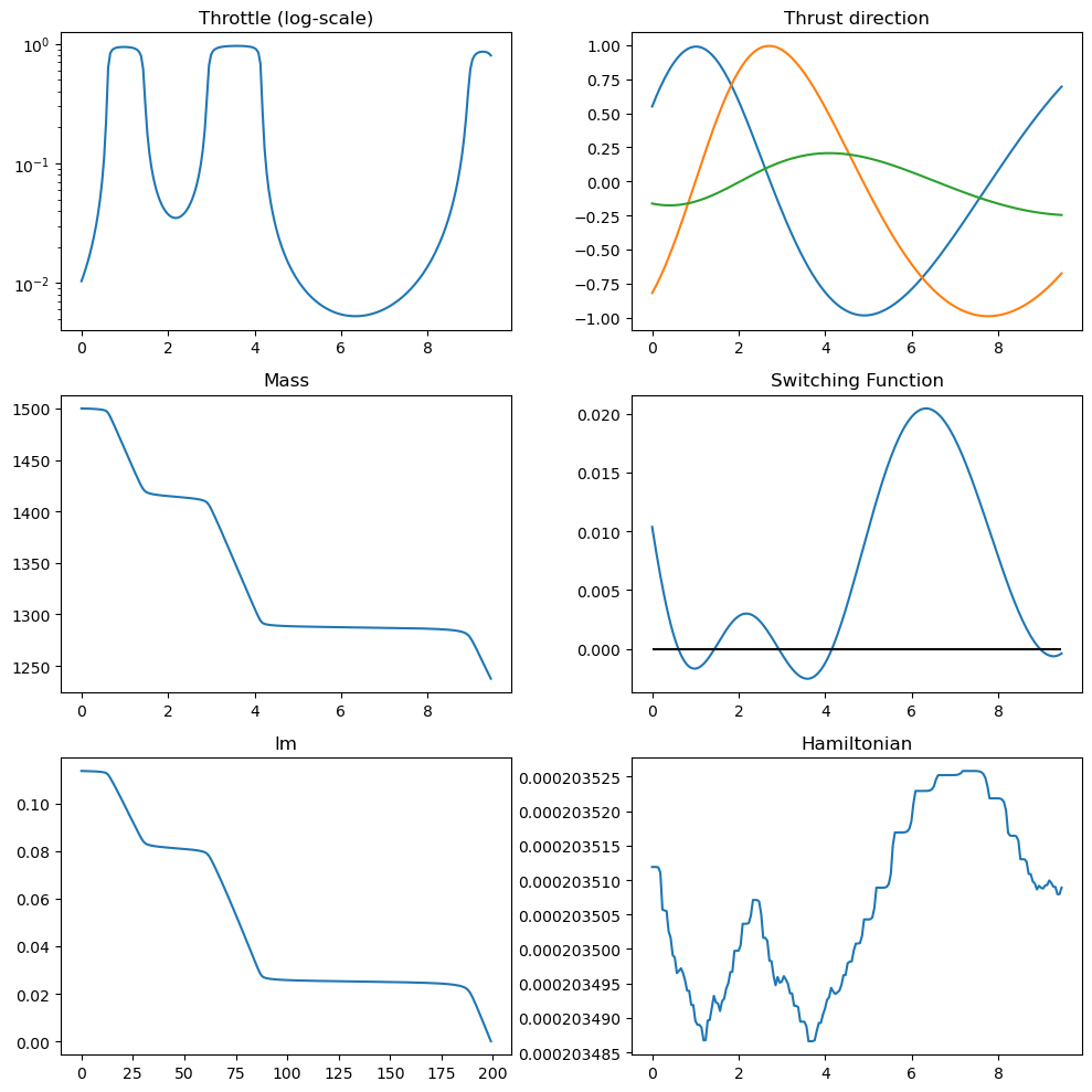
udp.plot_misc(pop.champion_x, N=200);

Continuation along the tangent direction

Here we decrease the \(\epsilon\) parameter exponentially and use as predictor the tangent vector along the solution curve. In our case the details are as follows. Assume the final constraints of TPBVB to be indicated with:

\[ \mathbf c(\mathbf \lambda, \epsilon) = 0 \]

where \(\mathbf \lambda = [\lambda_x, ..., \lambda_0]\). When \(\epsilon\) is changed slightly so must \(\mathbf \lambda\) change:

\[ \mathbf c(\mathbf \lambda + \delta\mathbf\lambda, \epsilon + \delta\epsilon) = 0 \]

In the linear world this is: $$

\frac{\partial \mathbf c}{\partial \mathbf \lambda}\delta\mathbf\lambda + \frac{\partial \mathbf c}{\partial \mathbf \epsilon}\delta\epsilon=0 $$

hence: $$

\delta \lambda = - \mathbf A^{-1}\mathbf B \delta \epsilon $$

where \(\mathbf A = \frac{\partial \mathbf c}{\partial \mathbf \lambda}\) and \(\mathbf B = \frac{\partial \mathbf c}{\partial \mathbf \epsilon}\).

Since the constraints are given directly on values of the final state, the matrices above can be computed seamlessly from a variational Taylor system. Only the last constraint \(|\lambda_0|\) is a exception but its gradient is also easily computed.

So lets build a variational integrator that helps here. pykep has the dynamics at hand in its pykep.ta module. We need to build a first order integrator to study variation of the variables: \([\lambda_x, \lambda_y, \lambda_z, \lambda_{vx}, \lambda_{vy},\lambda_{vz}, \lambda_{m}, \lambda_{0}, \epsilon]\).

sys = pk.ta.pc_dyn(pk.optimality_type.MASS)
lx, ly, lz, lvx, lvy, lvz, lm = hy.make_vars("lx", "ly", "lz", "lvx", "lvy", "lvz", "lm")
var_sys = hy.var_ode_sys(sys, [lx, ly, lz, lvx, lvy, lvz, lm, hy.par[4], hy.par[3]])
ta_var = hy.taylor_adaptive(var_sys, compact_mode = True)
ic_var = deepcopy(ta_var.state[14:])

We use the following small helper function to set the state for this new variational integrator, from some chromosome.

def set_ta_var_state(udp, x, ta_var, ic_var):
    # Preparing the numerical integration parameters
    ta_var.pars[0] = udp.mu
    ta_var.pars[1] = udp.c1
    ta_var.pars[2] = udp.c2
    ta_var.pars[3] = udp.eps
    ta_var.pars[4] = x[7]
    ta_var.time = 0.0

    # And initial conditions
    ta_var.state[:3] = udp.posvel0[0]
    ta_var.state[3:6] = udp.posvel0[1]
    ta_var.state[6] = udp.m0
    ta_var.state[7:14] = x[:7]
    ta_var.state[14:] = ic_var

import time
from copy import deepcopy
from IPython.display import clear_output

# No initial guess
first = True
epsilon = 1e-1
decrease_factor = 0.75

# Solve
while True:
    # Set the current epsilon in the udp (for later plotting)
    udp.eps = epsilon
    prob = pg.problem(udp)
    prob.c_tol = 1e-4

    # Random initial guess
    if first:
        # Creates a random ic population
        pop = pg.population(prob, 1)
        tstart_tot = time.time()
    # Use best chromosome from previous iteration
    else:
        pop = pg.population(prob)
        pop.push_back(predicted_chromosome)

    # Evolve
    tstart = time.time()
    pop = algo.evolve(pop)
    tend = time.time()

    # Compute error of fitness vector
    err = np.linalg.norm(pop.champion_f[1:])

    if prob.feasibility_f(pop.champion_f):
        clear_output(wait=True)
        print(
            f". Success!! | Error: {err:.2e} | CPU time: {tend-tstart:.2e} | Epsilon = {epsilon:.4e}"
        )
        
        # Stopping condition (desired epsilon reached)
        if epsilon < 1e-4:
            print(
                f"Desired epsilon reached ! | Error: {err:.2e} | CPU time: {tend-tstart:.2e} | Epsilon = {epsilon:.4e}"
            )
            predicted_chromosome = deepcopy(pop.champion_x)
            break

        # Save decision vector for current epsilon (which will be used as an initial guess in the next iteration)
        predicted_chromosome = deepcopy(pop.champion_x)
        first = False
        best_epsilon = epsilon
        
        # Compute tangent vector
        set_ta_var_state(udp, pop.champion_x, ta_var, ic_var)
        ta_var.propagate_until(udp.tof)

        # Find the tangent vector
        set_ta_var_state(udp, predicted_chromosome, ta_var, ic_var)
        ta_var.propagate_until(udp.tof);
        A = np.zeros((8,8))
        B = np.zeros((8,1))
        # Filling up the constraints on final state
        for i, component in enumerate([0,1,2,3,4,5,13]):
            slice = ta_var.get_vslice(order = 1, component = component)
            B[i,0] = ta_var.state[slice][-1]
            A[i, :] = ta_var.state[slice][:-1]
        # Filling up the constraints norm of lambda
        A[7,:] = 2*predicted_chromosome
        dx = np.ravel(- np.linalg.inv(A) @ B)

        # Save current epsilon (needed if next iteration fails)
        epsilon_previous = epsilon

        # Decrease epsilon
        f_decrease = decrease_factor
        predicted_chromosome = predicted_chromosome + dx * epsilon * (f_decrease-1)
        epsilon = epsilon * f_decrease

    else:
        clear_output(wait=True)
        print(
            f"x | Error: {err:.2e} | CPU time: {tend-tstart:.2e} | Epsilon = {epsilon:.4e}"
        )

        # If first iteration fails, try again with different initial guess
        if first:
            pass

        # Epsilon is too small, we need to increase it (halfway between previous and current)
        else:
            epsilon_previous_new = epsilon
            epsilon = epsilon + abs(epsilon_previous - epsilon) / 2
            epsilon_previous = epsilon_previous_new
tend_tot = time.time()
print(f"Total CPU time: {tend_tot - tstart_tot:.2e}")

. Success!! | Error: 2.08e-11 | CPU time: 1.45e-01 | Epsilon = 7.5254e-05
Desired epsilon reached ! | Error: 2.08e-11 | CPU time: 1.45e-01 | Epsilon = 7.5254e-05
Total CPU time: 3.15e+00

We obtained a smoother and faster method as our predictor is much better and allows for a more rapid exponential decrease (i.e. factor \(0.75\)).