Analysis of the Fitness Landscape
In this tutorial we want to show how to use the lanscape anlaysis module Dr. PyGMO for the analysis of the fitness function.
Instantiate Analysis Module
First, we need to instantiate the analysis class as follows:
from PyGMO import *

#We instantiate the optimization problem as usual. We will choose a 4-dimensional 2-objective
#problem.
prob=problem.kur(4)

#Now we instantiate the analysis class. In this case we will sample 500 points via sobol method
#and choose output to file.
inspector=util.analysis(prob, 500, method='sobol', output_to_file=True)
It is also an option to instantiate the class with an existing population object, for example:
pop=population(prob,500)
isl=island(algorithm.nsga_II(),pop)
isl.evolve(20)
pop_after_20_gen=isl.population

inspector_kur_20=util.analysis(pop_after_20_gen,output_to_file=True)
Tests on fitness functions
Now we can start launching some of the analysis. We will launch all of those that make sense for a 2-objective unconstrained problem.
inspector.f_distribution()

inspector.f_linearity_convexity()

#We will compute all regression properties for linear, quadratic and cubic regression, with
#and without interaction.
inspector.f_regression(degree=[1,1,2,2,3,3],interaction=[False,True,False,True,False,True])

inspector.f_sensitivity()

#The levelset test is very slow, we do not recommend launching it out of development purposes.
#Anyway this is an example so here it is. We will launch it using percentile 45 as threshold
#instead of the default 50, and only with 2-fold crossvalidation for tuning of svm.
inspector.levelset(threshold=45, k_tune=2)

#For the local searches, we will choose Nelder-Mead simplex algorithm. As it is a multi-objective
#problem, we will also choose a decomposition method, for instance weighted with uniform weights.
#To keep it short, we will only show properties of the best 3 clusters instead of the default 10.
#We will also generate a scatter plot for dimensions x1 and x2.
inspector.local_search(clusters_to_show=3, scatter_plot_dimensions=[1,2],\
algo=algorithm.gsl_nm(), decomposition_method='weighted', weights='uniform')

#Being only a 2-objective problem, we probably will not obtain dimensionality reduction, but we
#will launch this test all the same to look into the f-correlation matrix.
inspector.f_correlation()
The output should be something like this:
===============================================================================
ANALYSIS
===============================================================================
-------------------------------------------------------------------------------
PROBLEM PROPERTIES
-------------------------------------------------------------------------------
Problem name: Kursawe's study
Global dimension: 4
Integer dimension: 0
Fitness dimension: 2
Constraints dimension: 0
Inequality constraints dimension: 0
Lower bounds: [-5, -5, -5, -5]
Upper bounds: [5, 5, 5, 5]
Constraints tolerance: []
-------------------------------------------------------------------------------
SAMPLED [500] POINTS VIA sobol METHOD FOR THE SUBSEQUENT TESTS
--------------------------------------------------------------------------------
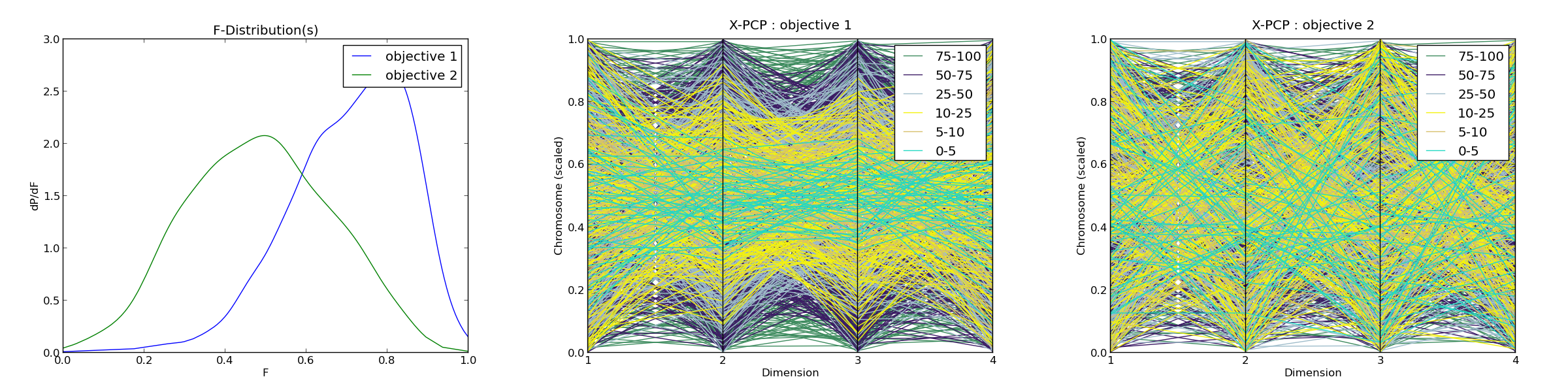
F-DISTRIBUTION FEATURES (2 OBJECTIVES)
--------------------------------------------------------------------------------
Fitness magnitude :
Min : [-30.0, -10.636]
Max : [-8.118, 27.962]
Peak-to-peak (scale factor) : [21.882, 38.598]
Fitness distribution :
Mean : [0.706, 0.484]
Standard deviation : [0.146, 0.176]
Percentiles :
5 : [0.449, 0.208]
10 : [0.513, 0.256]
25 : [0.614, 0.358]
50 : [0.728, 0.483]
75 : [0.818, 0.613]
Skew : [-0.725, 0.016]
Kurtosis : [0.592, -0.499]
Number of peaks of f-distribution : [1, 1]
*F-distribution plot : <figure_1.png>
*X-PCP plot obj.1 : <figure_2.png>
*X-PCP plot obj.2 : <figure_3.png>
-------------------------------------------------------------------------------
PROBABILITY OF LINEARITY AND CONVEXITY
-------------------------------------------------------------------------------
Number of pairs of points used : [500]
Probability of linearity : [0.0, 0.0]
Probability of convexity : [0.938, 0.544]
Mean deviation from linearity : [0.098, 0.201]
-------------------------------------------------------------------------------
F-REGRESSION
-------------------------------------------------------------------------------
OBJECTIVE 1 :
DEGREE F R2 R2adj RMSE R2pred PRESS-RMSE
1 0.051 0.001 -0.01 0.147 -0.021 0.147
1(i) 0.051 0.001 -0.01 0.147 -0.021 0.147
2 253.291 0.887 0.883 0.05 0.879 0.051
2(i) 253.291 0.887 0.883 0.05 0.879 0.051
3 181.939 0.927 0.922 0.041 0.919 0.041
3(i) 181.939 0.927 0.922 0.041 0.919 0.041
OBJECTIVE 2 :
DEGREE F R2 R2adj RMSE R2pred PRESS-RMSE
1 0.384 0.004 -0.006 0.177 -0.019 0.178
1(i) 0.384 0.004 -0.006 0.177 -0.019 0.178
2 3.018 0.085 0.057 0.171 0.023 0.174
2(i) 3.018 0.085 0.057 0.171 0.023 0.174
3 1.823 0.113 0.051 0.172 -0.03 0.179
3(i) 1.823 0.113 0.051 0.172 -0.03 0.179
-------------------------------------------------------------------------------
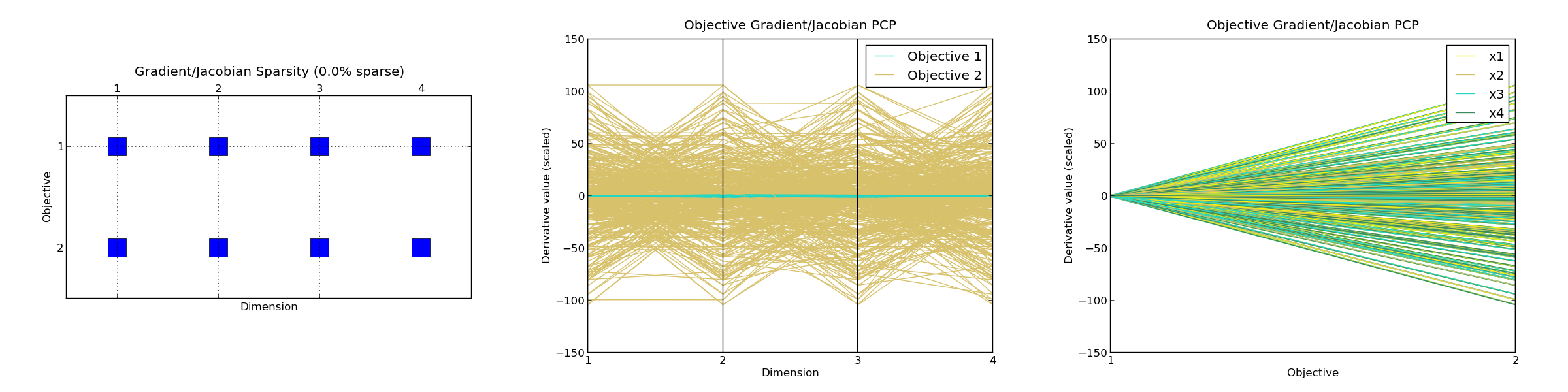
F-SENSITIVITY
-------------------------------------------------------------------------------
Number of points used : [500]
OBJECTIVE 1 :
Percentiles : | 0 | 25 | 50 | 75 | 100 |
Gradient norm : | 0.0 | 0.831 | 0.951 | 1.114 | 1.734 |
|dFx|_max/|dFx|_min : | 1.387 | 2.71 | 4.073 | 8.895 | inf |
Hessian conditioning : | 2.0 | 3.401 | 5.482 | 10.931 | 2048.592|
Gradient sparsity : [0.0]
Fraction of points with PD hessian : [0.002]
Fraction of points with PSD (not PD) hessian : [0.0]
OBJECTIVE 2 :
Percentiles : | 0 | 25 | 50 | 75 | 100 |
Gradient norm : | 0.0 | 36.605 | 60.743 | 85.195 | 151.023 |
|dFx|_max/|dFx|_min : | 1.014 | 10.043 | 28.023 | 89.425 | inf |
Hessian conditioning : | 1.0 | 45.903 | 276.67 | 974.877 |46518.448|
Gradient sparsity : [0.0]
Fraction of points with PD hessian : [0.064]
Fraction of points with PSD (not PD) hessian : [0.0]
*Gradient/Jacobian sparsity plot : <figure_4.png>
*Objective Gradient/Jacobian PCP plot : <figure_5.png>
*Objective Gradient/Jacobian PCP plot (inverted) : <figure_6.png>
-------------------------------------------------------------------------------
LEVELSET FEATURES
-------------------------------------------------------------------------------
Percentile 45 :
Mean Misclassification Errors
Linear Kernel : [0.45, 0.45]
Quadratic Kernel : [0.242, 0.464]
Non-Linear Kernel (RBF): [0.054, 0.428]
P-Values :
Linear/Quadratic : [0.0, 0.438]
Linear/Nonlinear : [0.0, 0.028]
Quadratic/Nonlinear : [0.0, 0.067]
--------------------------------------------------------------------------------
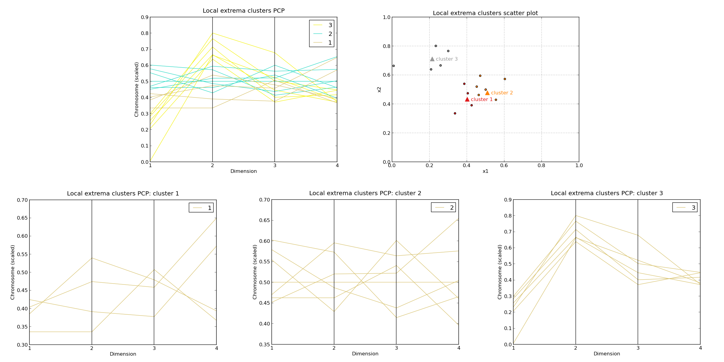
LOCAL SEARCH
--------------------------------------------------------------------------------
WARNING: get_local_extrema is decomposing multi-objective problem by means of
weighted method, with uniform weight vector!
Local searches performed : 1000
Quartiles of CPU time per search [ms]: 7.0 / 19.0 / 26.0 / 36.0 / 51.0
Number of clusters identified : 159
Cluster properties (max. best 3 clusters) :
Cluster n. 1 :
Size: 4.0 , 0.4 %
Cluster X_center : [0.402, 0.433, 0.442, 0.498]
Mean objective value : [0.275, 0.121]
F(X_center) : [0.221, 0.168]
Cluster span in F : [0.202, 0.134]
Cluster radius in X : 0.159
Radius of attraction : 0.188
Cluster n. 2 :
Size: 7.0 , 0.7 %
Cluster X_center : [0.509, 0.478, 0.51, 0.516]
Mean objective value : [0.131, 0.276]
F(X_center) : [0.061, 0.297]
Cluster span in F : [0.207, 0.203]
Cluster radius in X : 0.157
Radius of attraction : 0.172
Cluster n. 3 :
Size: 6.0 , 0.6 %
Cluster X_center : [0.214, 0.712, 0.487, 0.406]
Mean objective value : [0.508, 0.082]
F(X_center) : [0.47, 0.436]
Cluster span in F : [0.208, 0.162]
Cluster radius in X : 0.219
Radius of attraction : 0.216
*Cluster PCP plot (global) : <figure_7.png>
*Cluster PCP plot (cluster n.1) : <figure_8.png>
*Cluster PCP plot (cluster n.2) : <figure_9.png>
*Cluster PCP plot (cluster n.3) : <figure_10.png>
*Cluster scatter plot (dimensions [1, 2]) : <figure_11.png>
--------------------------------------------------------------------------------
OBJECTIVE CORRELATION
--------------------------------------------------------------------------------
Critical objectives from first PCA :     [1, 2]
Eigenvalues   Relative contribution                   Eigenvectors
   0.723             36.128%                        [-0.707, 0.707]
   1.277             63.872%                         [0.707, 0.707]
Objective correlation matrix :
     [  1.0    0.277  ]
     [ 0.277    1.0   ]