PADE: a parallel MOEA-D algorithm
In this tutorial we will learn how to use PADE to solve a multi-objective problem. PADE transforms a multi-objective problem into N single-objective ones, where N is the population size. It does that using the Decomposition meta problem. It then solve each problem in parallel using a given single objective algorithm. The population provided at the end of the evolution will be the union of the solutions to each single-objective problem.
Let start using PADE to solve the popular multi-objective benchmark problem ZDT1.
In [1]: from PyGMO import *
In [2]: prob = problem.zdt(1)
In [3]: alg = algorithm.pade()
In [4]: pop = population(prob, 100)
In [5]: pop = alg.evolve(pop)
In [6]: pop.plot_pareto_fronts()
We will get the following

Each point on the pareto front corresponds to the solution to a single-objective problem. In order for the point to be well spread is then crucial to choose the proper decomposition method and the proper weight vectors. It is possible to do that as follow
In [7]: alg = algorithm.pade(decomposition = problem.decompose.BI, weights=algorithm.pade.GRID)
In [8]: pop = alg.evolve(pop)
In [9]: pop.plot_pareto_fronts()
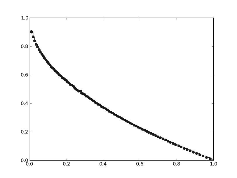
As we can see the points on the pareto front are much better spread.
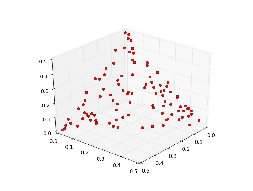
In the following plots we see how different weight generation methods perform on the 3-objective benchmark problem DTLZ1. First we will use a RANDOM weight generation.
In [1]: from PyGMO import *
In [2]: alg = algorithm.pade(decomposition = problem.decompose.BI, weights=algorithm.pade.RANDOM)
In [3]: prob = problem.dtlz(1)
In [4]: pop = population(prob,100)
In [5]: pop = alg.evolve(pop)
In [6]: prob.plot(pop)
Let’s now try generating the weight vectors with the GRID method
In [7]: alg = algorithm.pade(decomposition = problem.decompose.BI, weights=algorithm.pade.GRID)
In [8]: pop = population(prob,100)
In [9]: pop = alg.evolve(pop)
---------------------------------------------------------------------------
ValueError                                Traceback (most recent call last)
<ipython-input-10-1eb0f083e7c3> in <module>()
----> 1 pop = alg.evolve(pop)

ValueError: /home/mambro/qtcreator_workspace/pagmo-code/src/algorithm/pade.cpp,183: Invalid population size. Select 91 or 105..
As we can see from the error message we cannot use any population size. The error message will suggest us the two accepted values closer to the one we wanted. Let’s then choose 105.
In [10]: pop = population(prob,105)
In [11]: pop = alg.evolve(pop)
In [12]: prob.plot(pop)
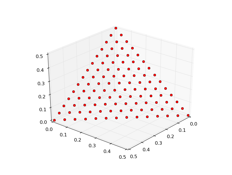
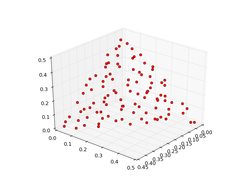
As we can see the front is much better spread. The only drawback of the GRID method is that we are not free to choose any population size. To have a better spread than the one obtained with the RANDOM method but still be able to choose any population size, we can use the LOW_DISCREPANCY method.
In [13]: alg = algorithm.pade(decomposition = problem.decompose.BI, weights=algorithm.pade.LOW_DISCREPANCY)
In [14]: pop = population(prob,100)
In [15]: pop = alg.evolve(pop)
In [16]: prob.plot(pop)
We now introduce two more interesting features of PADE.
It is possible to choose which single-objective algorithm to use to solve each single-objective problem the original problem is decomposed into, in the following way
In [1]: alg = algorithm.pade(solver = algorithm.jde(50))
Moreover, as said at the beginning of the tutorial, PADE solves the single-objective problems in parallel. It is possible to set how many threads to run. This should be ideally equal to the number of logic cores available in the machine which runs the code.
In [2]: alg = algorithm.pade(max_parallelism = 8)