Indirect methods IV (minimum time, MEE)

This notebook presents a minimum-time low-thrust transfer solved with an indirect method in modified equinoctial elements (MEE).

As in the Cartesian time-optimal case, PMP yields full throttle in this formulation, so homotopy on \(\epsilon\) is not needed.

For comparison, see Cartesian time-optimal notebook and equinoctial mass-optimal notebook.

import pykep as pk
import numpy as np
import heyoka as hy
import pygmo as pg
import pygmo_plugins_nonfree as ppnf
import time

from matplotlib import pyplot as plt

---------------------------------------------------------------------------
ModuleNotFoundError                       Traceback (most recent call last)
Cell In[1], line 5
      1 import pykep as pk
      2 import numpy as np
      3 import heyoka as hy
      4 import pygmo as pg
----> 5 import pygmo_plugins_nonfree as ppnf
      6 import time
      7 
      8 from matplotlib import pyplot as plt

ModuleNotFoundError: No module named 'pygmo_plugins_nonfree'

Manual construction of the TPBVP

We consider a spacecraft of mass \(m\) under central gravity with parameter \(\mu\), equipped with low-thrust propulsion of maximum thrust \(T_{\max}=c_1\) and effective exhaust velocity \(c_2=I_{sp}g_0\).

The state is \([p,f,g,h,k,L,m]^T\), where \([p,f,g,h,k,L]^T\) are prograde modified equinoctial elements (see Elements page).

The controlled dynamics are

\[\begin{split} \begin{array}{l} \dot p = \sqrt{\frac p\mu} \frac{2p}{w} i_t\, c_1 \frac{u}{m} \\ \dot f = \sqrt{\frac p\mu} \left\{i_r \sin L + \left[ (1+w)\cos L + f \right] \frac{i_t}{w} - (h\sin L-k\cos L)\frac{g i_n}{w} \right\} c_1\frac{u}{m} \\ \dot g = \sqrt{\frac p\mu} \left\{ - i_r\cos L + \left[ (1+w)\sin L + g \right] \frac{i_t}{w} + (h\sin L-k\cos L)\frac{f i_n}{w} \right\} c_1\frac{u}{m} \\ \dot h = \sqrt{\frac p\mu} \frac{s^2 i_n}{2w}\cos L\, c_1\frac{u}{m} \\ \dot k = \sqrt{\frac p\mu} \frac{s^2 i_n}{2w}\sin L\, c_1\frac{u}{m} \\ \dot L = \sqrt{\frac p\mu}\left\{\mu\left(\frac wp\right)^2 + \frac{1}{w}\left(h\sin L-k\cos L\right)i_n c_1\frac{u}{m} \right\} \\ \dot m = -\frac{c_1}{c_2}u \end{array} \end{split}\]

with \(w = 1 + f\cos L + g\sin L\), \(s^2 = 1 + h^2 + k^2\), control constraints \(0\le u\le1\), and \(\hat{\mathbf i}_{\tau}=[i_r,i_t,i_n]^T\) such that \(\|\hat{\mathbf i}_{\tau}\|=1\).

A compact form is

\[\begin{split} \left\{ \begin{array}{l} \dot{\mathbf x} = \frac{c_1u(t)}{m}\mathbf B(\mathbf x)\hat{\mathbf i}_{\tau} + \mathbf D(\mathbf x) \\ \dot m = -\frac{c_1}{c_2}u(t) \end{array} \right., \end{split}\]

where

\[\begin{split} \sqrt{\frac{\mu}{p}}\mathbf B(\mathbf x)= \left[ \begin{array}{ccc} 0 & \frac{2p}{w} & 0 \\ \sin L & \frac{(1+w)\cos L + f}{w} & -\frac{g}{w}(h\sin L-k\cos L) \\ -\cos L & \frac{(1+w)\sin L + g}{w} & \frac{f}{w}(h\sin L-k\cos L) \\ 0 & 0 & \frac{s^2}{2w}\cos L \\ 0 & 0 & \frac{s^2}{2w}\sin L \\ 0 & 0 & \frac{1}{w}(h\sin L-k\cos L) \end{array} \right], \end{split}\]

and

\[ \mathbf D(\mathbf x)=\left[0,0,0,0,0,\sqrt{\frac{\mu}{p^3}}w^2\right]^T. \]

Using heyoka, we now define symbolic variables for states, controls, and costates.

# State variables
p, f, g, h, k, L, m = hy.make_vars("p", "f", "g", "h", "k", "L", "m")
# Costate variables
lp, lf, lg, lh, lk, lL, lm = hy.make_vars(
    "lp", "lf", "lg", "lh", "lk", "lL", "lm"
)
# Control variables: throttle and RTN thrust direction
u, i_r, i_t, i_n = hy.make_vars("u", "ir", "it", "in")

To keep the derivation readable, we define compact expressions and vectorized groupings.

# Reusable scalar expressions
w = 1 + f * hy.cos(L) + g * hy.sin(L)
s2 = 1 + h * h + k * k
B = np.array(
    [
        [0, 2 * p / w, 0.0],
        [
            hy.sin(L),
            ((1 + w) * hy.cos(L) + f) / w,
            -g / w * (h * hy.sin(L) - k * hy.cos(L)),
        ],
        [
            -hy.cos(L),
            ((1 + w) * hy.sin(L) + g) / w,
            f / w * (h * hy.sin(L) - k * hy.cos(L)),
        ],
        [0, 0, s2 / w / 2.0 * hy.cos(L)],
        [0, 0, s2 / w / 2.0 * hy.sin(L)],
        [0, 0, 1.0 / w * (h * hy.sin(L) - k * hy.cos(L))],
    ]
) * hy.sqrt(p / hy.par[0])

D = np.array([0.0, 0.0, 0.0, 0.0, 0.0, hy.sqrt(hy.par[0] / p / p / p) * w * w])

i_vers = np.array([i_r, i_t, i_n])
lx = np.array([lp, lf, lg, lh, lk, lL])

The dynamics can then be written as:

# Dynamics
fx = np.dot(B, i_vers) * u * hy.par[1] / m + D
fm = - hy.par[1] / hy.par[2] * u

We introduce the Hamiltonian (\(\mathbf x\) is the full state and \(\boldsymbol\lambda\) the full costate):

\[ \mathcal H(\mathbf x, \boldsymbol\lambda, \mathbf u) = \boldsymbol\lambda_x\cdot\mathbf f_x + \lambda_m f_m + \lambda_0\frac{c_1}{c_2}. \]

# Time-optimal Hamiltonian
H_full = (lx @ fx + lm * fm + hy.par[4] * hy.par[1] / hy.par[2])
# Switching function rho (negative in this setting, giving full throttle)
BTlam = B.T@lx 
BTlam_norm = hy.sqrt(BTlam @ BTlam)
rho = - hy.par[2] * BTlam_norm / m / hy.par[4] - lm / hy.par[4]

Constants are passed as heyoka parameters in the order \([\mu, c_1, c_2, \epsilon, \lambda_0]\), with \(c_1=T_{\max}\) and \(c_2=I_{sp}g_0\).

As in the Cartesian time-optimal notebook, \(\epsilon\) is retained only for API consistency with the mass-optimal formulation and does not enter the objective in this case. \(\lambda_0\) can be used for normalization but does not change the nature of the minimum-time objective.

And write the resulting Hamiltonian system:

\[\begin{split} \left\{ \begin{array}{l} \dot{\mathbf x} = \frac{\partial \mathcal H}{\partial \mathbf \lambda} \\ \dot{\mathbf \lambda} = - \frac{\partial \mathcal H}{\partial \mathbf x} \\ \end{array}\right. \end{split}\]

# Augmented equations of motion
rhs = [
    hy.diff(H_full, var)
    for var in [lp, lf, lg, lh, lk, lL, lm, p, f, g, h, k, L, m]
]
for j in range(7, 14):
    rhs[j] = -rhs[j]

Pontryagin’s minimum principle requires pointwise minimization over admissible controls

\[ \mathbf u^*(t)=\arg\min_{\mathbf u\in\mathcal U}\mathcal H(\mathbf x,\boldsymbol\lambda,\mathbf u), \]

with \(\mathcal U=\{(u,\hat{\mathbf i}_{\tau})\,|\,0\le u\le 1,\ \|\hat{\mathbf i}_{\tau}\|=1\}\).

For this time-optimal problem, the minimizer is:

# We apply Pontryagin minimum principle (primer vector and u^* = 2eps / (rho + 2eps + sqrt(rho^2+4*eps^2)))
argmin_H_full = {
    i_r: -BTlam[0] / BTlam_norm,
    i_t: -BTlam[1] / BTlam_norm,
    i_n: -BTlam[2] / BTlam_norm,
    u: hy.expression(1.)
}

After substitution, controls become explicit functions of state and costate and the augmented dynamics close in \((\mathbf x,\boldsymbol\lambda)\).

rhs = hy.subs(rhs, argmin_H_full)

# We also build the Hamiltonian as a function of the state / co-state only
# (i.e. no longer of controls now solved thanks to the minimum principle)
H = hy.subs(H_full, argmin_H_full)

The next block instantiates the heyoka integrator and helper evaluators used for the shooting implementation.

# Compile Hamiltonian evaluator (pars = [mu, c1, c2, eps, lambda0]; eps unused here)
H_func = hy.cfunc([H], [p, f, g, h, k, L, m , lp, lf, lg, lh, lk, lL, lm ])
# Compile optimal throttle evaluator
u_func = hy.cfunc(
    [argmin_H_full[u]], [p, f, g, h, k, L, m , lp, lf, lg, lh, lk, lL, lm ]
)
# Compile switching-function evaluator
rho_func = hy.cfunc([rho], [p, f, g, h, k, L, m , lp, lf, lg, lh, lk, lL, lm ])
# Compile optimal RTN thrust-direction evaluator
i_vers_func = hy.cfunc(
    [argmin_H_full[i_r], argmin_H_full[i_t], argmin_H_full[i_n]], [p, f, g, h, k, L, m , lp, lf, lg, lh, lk, lL, lm ]
)
# Assemble Taylor adaptive integrator
full_state = [p, f, g, h, k, L, m , lp, lf, lg, lh, lk, lL, lm ]
sys = [(var, dvar) for var, dvar in zip(full_state, rhs)]
ta = hy.taylor_adaptive(sys, state=[1.0] * 14, compact_mode=True)

# note that the dynamics does not depend on hy.par[4] so all those equations will be zero. 
# we nevertheless use hy.par[4] for consistency with the mass optimal case which can be handy.
var_sys = hy.var_ode_sys(sys, args = [lp,lf,lg,lh,lk,lL,lm, hy.par[4]])
ta_var = hy.taylor_adaptive(var_sys, compact_mode=True)

Constructing the TPBVP using pykep

pykep provides pre-assembled components equivalent to the manually derived objects above.

In practice, these are preferred for robust workflows, while manual derivations remain useful for understanding and debugging.

# The Taylor integrator
ta = pk.ta.get_peq(1e-16, pk.optimality_type.TIME)
# The Variational Taylor integrator
ta_var = pk.ta.get_peq_var(1e-16, pk.optimality_type.TIME)
# The Hamiltonian
H_func = pk.ta.get_peq_H_cfunc(pk.optimality_type.TIME)
# The switching function
SF_func = pk.ta.get_peq_SF_cfunc(pk.optimality_type.TIME)
# The magnitude of the throttle
u_func = pk.ta.get_peq_u_cfunc(pk.optimality_type.TIME)
# The thrust direction
i_vers_func = pk.ta.get_peq_i_vers_cfunc(pk.optimality_type.TIME)
# The dynamics cfunc
dyn_func = pk.ta.get_peq_dyn_cfunc(pk.optimality_type.TIME)

Solving in single shooting

The previous section was primarily pedagogical. From here onward, we use dedicated pykep classes to assemble and solve the shooting problem.

As a test case, we use the same baseline transfer as in the equinoctial mass-optimal notebook.

# Testcase 1 
source=pk.planet(pk.udpla.jpl_lp("earth"))
target=pk.planet(pk.udpla.jpl_lp("mars"))

tof_guess = 250
mu = pk.MU_SUN
eps = 1e-5
T_max = 6.
Isp = 3000
m0 = 1500
n_rev=0

We instantiate the shooting method using the UDP provided by pykep:

# Factory for the pygmo udp.
def prob_factory(T_max, tof_guess):
    udp = pk.trajopt.pontryagin_equinoctial_time(
        source=source,
        target=target,
        tof_guess=tof_guess,
        t0 = pk.epoch(400),
        lambda0 = None,  # We normalize the costates
        T_max=T_max,
        veff=3000*pk.G0,
        m0=1500,
        n_rev=0,
        L=pk.AU,
        MU=pk.MU_SUN,
        MASS=1500,
        with_gradient=True,
        taylor_tolerance=1e-10, # lower tolerance for the Taylor integrator since the problem is easy
        taylor_tolerance_var=1e-10
    )
    udp.ta = ta
    prob = pg.problem(udp)
    prob.c_tol = 1e-6
    return prob

prob = prob_factory(0.6, 250)
sparsity = prob.gradient_sparsity()
udp = prob.extract(pk.trajopt.pontryagin_equinoctial_time)

The resulting TPBVP can be solved with interior-point optimizers or root-finding methods on boundary residuals.

Here we use IPOPT (via pagmo) and a MINPACK wrapper (via scipy.optimize.root).

ip = pg.ipopt()
ip.set_numeric_option("tol", 1e-9)  # Relative convergence tolerance
ip.set_integer_option("max_iter", 50)  # Maximum iterations
ip.set_integer_option("print_level", 0)  # Suppress IPOPT console output
ip.set_string_option(
    "sb", "yes"
)
ip.set_string_option(
    "nlp_scaling_method", "none"
)  # Disable IPOPT automatic scaling
ip.set_string_option(
    "mu_strategy", "adaptive"
)  # Adaptive barrier update strategy
ipopt = pg.algorithm(ip)

MINPACK is available via scipy and is missing in the current pygmo version, but we can quickly provide a wrapper as a UDA:

class my_solver:
    def __init__(self, gradient):
        self.gradient = gradient
    def evolve(self, pop: pg.population):
        from scipy.optimize import root
        prob = pop.problem
        x0 = pop.champion_x
        n = prob.get_nx()
        if self.gradient:
            def dense_grad(x):
                G = np.zeros((n,n))
                G[sparsity[:, 0], sparsity[:, 1]] = prob.gradient(x)
                return G.reshape(n,n)
            res = root(lambda x: [0] +  list(prob.fitness(x)[1:]), x0, method="hybr", tol=1e-8, options = {"factor": 1., "diag": [1]*(n)}, jac=dense_grad)  # factor=1 is very important for convergence
        else:
            res = root(lambda x: [0] +  list(prob.fitness(x)[1:]), x0, method="hybr", tol=1e-8, options = {"factor": 1., "diag": [1]*(n)})  # factor=1 is very important for convergence
        pop.set_x(0, res["x"])
        return pop
    def get_name(self):
        return "Minpack hybrd routine"

minpack = pg.algorithm(my_solver(False))
minpack_g = pg.algorithm(my_solver(True))

We use a multi-start strategy, which is generally good practice for indirect shooting due to sensitivity to initialization. In this easy case, multiple starts are mainly used to report robustness.

def multistart(algo, n_trials=50):
    masses = []
    xs = []
    total_time = 0.0
    success=0

    for i in range(n_trials):
        pop = pg.population(prob,1)
        time_start = time.time()
        pop = algo.evolve(pop)
        time_end = time.time()
        total_time += time_end - time_start
        if prob.feasibility_f(pop.champion_f):
            print(".", end="")
            udp.fitness(pop.champion_x)
            xs.append(pop.champion_x)
            masses.append(udp.ta.state[6])
            success+=1
        else:
            print("x", end="")
    if masses:
        print(f"\nFinal mass is: {masses[0]*udp.MASS}")
        print(f"Total time to success: {total_time:.3f} seconds")
        print(f"Number of successes: {success} over {n_trials} trials ({success/n_trials*100:.1f} %)")
    else:
        print("\nNo success")
    return pop

pop = multistart(ipopt, n_trials=10)

...x.....x
Final mass is: 1049.4338611857288
Total time to success: 12.165 seconds
Number of successes: 8 over 10 trials (80.0 %)

pop = multistart(minpack_g, n_trials=10)

...x......
Final mass is: 1049.43386119149
Total time to success: 2.154 seconds
Number of successes: 9 over 10 trials (90.0 %)

ax = udp.plot(pop.champion_x)
ax.view_init(90,0)

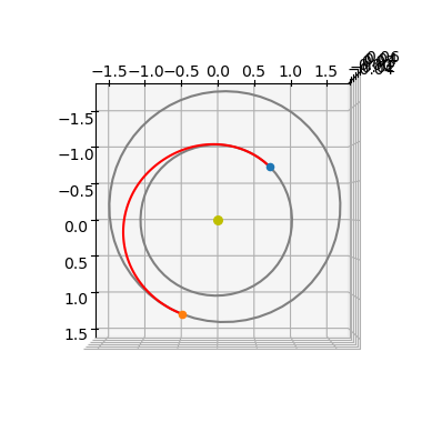
Thrust arcs are indicated with a red color, ballistic with blue.

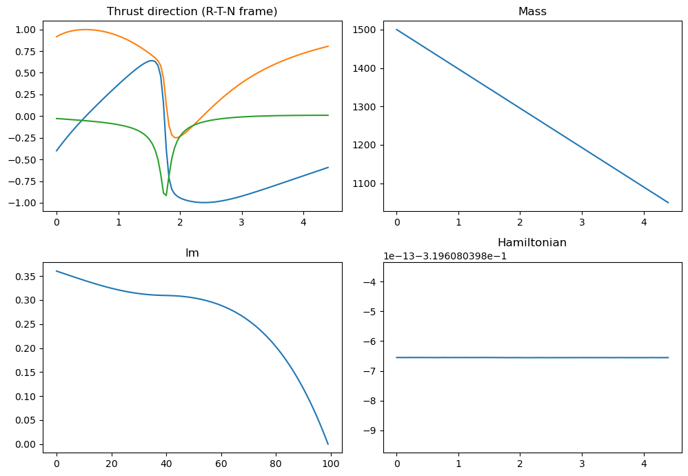
udp.plot_misc(pop.champion_x);