Multiple impulses: planet to planet transfer

In this tutorial, we use the pykep.trajopt.pl2pl_N_impulses to study a single direct transfer between planets.

The encoding is original with pykep and makes use of a decision vector (chromosome) in the form:

\[ \mathbf x = [t_0,T] + \underbrace{[\alpha_0,u_0,v_0,\Delta V_0] + [\alpha_1,u_1,v_1,\Delta V_1] + ...}_{\text{propagations}} + \underbrace{[\alpha_{N-1}]}_{\text{Lambert}} + \underbrace{([t_f])}_{\text{Optional phase term}} \]

to define an \(N\) impulse trajectory starting at \(t_0\) at the departure planet with a \(\Delta V_0\) and arriving at the target planet with a \(\Delta V_{N-1}\) and applying the remaining \(\Delta V_i\) at epochs encoded using the \(\alpha\)-encoding for times (see Multiple Gravity Assist (MGA)).

This optimization problem is a nice tool to visualize and study the famous “How many impulses?” question which has a very complicated answer in general.

We start, as often, with some fundamental imports:

import pykep as pk
import numpy as np
import pygmo as pg

We define the problem as an Earth-Venus transfer. We set the transfer time as fixed as well as the departure epoch.

start = pk.planet(pk.udpla.jpl_lp("earth"))
target = pk.planet(pk.udpla.jpl_lp("venus"))

tof_bounds = [360.0, 360.0]
DV_max_bounds = [0.0, 4]
phase_free = False
multi_objective = False
t0_bounds = [140, 140.]

udp3 = pk.trajopt.pl2pl_N_impulses(
    start=start,
    target=target,
    N_max=3,
    tof_bounds=tof_bounds,
    phase_free=phase_free,
    multi_objective=multi_objective,
    t0_bounds=t0_bounds,
    DV_max_bounds=DV_max_bounds
)

def solve(udp, N=20):
    # We use CMA-ES 
    uda = pg.cmaes(4500, force_bounds=True, sigma0=0.5, ftol=1e-4)
    # But if you prefer a self adaptive version of differential evolution thats also OK.
    #uda = pg.sade(2500, ftol=1e-4, xtol=1e-4)
    algo = pg.algorithm(uda)

    print("Multi-start:")

    res = list()
    for i in range(N):
        pop = pg.population(udp, 20)
        pop = algo.evolve(pop)
        res.append([pop.champion_f, pop.champion_x])
        print(i, pop.champion_f[0], end= '\r')
        

    best_x = sorted(res, key =  lambda x: x[0][0])[0][1]

    print(f"\nThe best solution found has a DV of {udp.fitness(best_x)[0]/1000:.5e} km/s")
    return best_x

best_x_3 = solve(udp3)

Multi-start:
0 6312.58212984
1 6015.33207582
2 5986.38946166
3 5986.38945646
4 6312.58212984

5 6312.58212984
6 5986.38946673
7 5986.38946602
8 6015.33207582
9 6015.33207584
10 5986.38946242
11 5986.38945651

12 6312.58212984
13 6015.33207579
14 6312.58212984
15 6312.58212984
16 6312.58212984

17 6148.72614657
18 6015.3320758
19 5986.38945984
The best solution found has a DV of 5.98639e+00 km/s

We can easily visualize the solution:

def visualise(udp, best_x):
    import matplotlib.pyplot as plt
    import numpy as np

    # Create the figure and define the grid
    fig = plt.figure(figsize=(10, 10))
    gs = fig.add_gridspec(
        2, 2, width_ratios=[2, 1], height_ratios=[1, 1], wspace=0.01, hspace=0.01
    )

    # Top view (spans rows and columns)
    ax1 = fig.add_subplot(gs[:, 0], projection="3d")
    udp.plot(best_x, ax=ax1)
    ax1.view_init(90, 0)
    ax1.axis("off")

    # Ecliptic view 1
    ax1 = fig.add_subplot(gs[0, 1], projection="3d")
    udp.plot(best_x, ax=ax1)
    ax1.view_init(0, 0)
    ax1.axis("off")

    # Ecliptic view 2
    ax1 = fig.add_subplot(gs[1, 1], projection="3d")
    udp.plot(best_x, ax=ax1)
    ax1.view_init(0, 90)
    ax1.axis("off")
    return fig


visualise(udp3, best_x_3);

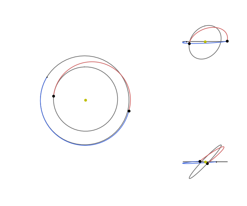
… and quickly investigate a human readable format for the solution found.

udp3.pretty(best_x_3)

Total DV (m/s):  5986.389456458053
Dvs (m/s):  [219.51985100028682, 2899.3203407504793, 2867.5492647072874]
Total DT (days):  360.0
Tofs (days):  [205.9431149414002, 154.05688505859976]

Are more impulses needed?

In the previous design we allowed maximum 3 impulses, but would more impulse be needed? We can quickly answer this question for this specific case by looking at the primer vector.

ax, (grid, p) = udp3.plot_primer_vector(best_x_3)

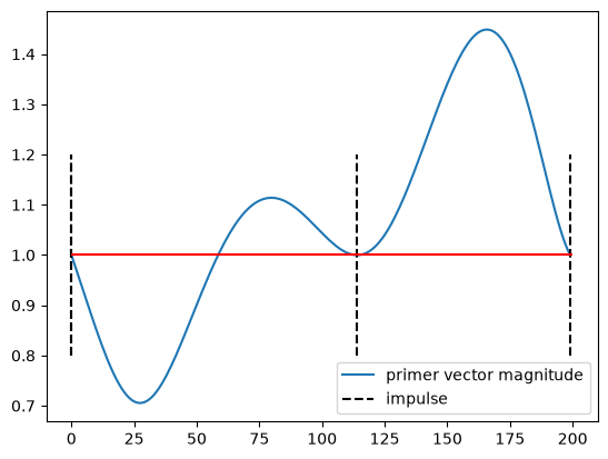
… the primer vector goes above one this trajevtory IS NOT OPTIMAL. We need more impulses. Lets add one.

udp4 = pk.trajopt.pl2pl_N_impulses(
    start=start,
    target=target,
    N_max=4,
    tof_bounds=tof_bounds,
    phase_free=phase_free,
    multi_objective=multi_objective,
    t0_bounds=t0_bounds,
    DV_max_bounds=DV_max_bounds
)

best_x_4 = solve(udp4, N=20)

Multi-start:

0 5986.44298923

1 5986.44847542
2 6015.44394313

3 5986.44294879
4 5986.38945627

5 6015.33207595
6 5986.38945626

7 5937.92761602
8 5986.38945625

9 5986.38945634
10 5938.64538643

11 5986.38945626
12 5986.38945641
13 5986.38945625

14 6015.33207589

15 5986.44295491
16 5986.38945626

17 5986.38945626

18 5986.44293755

19 5969.77850114
The best solution found has a DV of 5.93793e+00 km/s

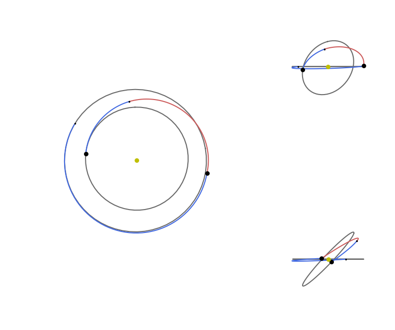
visualise(udp4, best_x_4);

udp4.pretty(best_x_4)

Total DV (m/s):  5937.927616024613
Dvs (m/s):  [197.63077785108803, 2732.0388547423236, 230.71703539845916, 2777.540948032742]
Total DT (days):  360.0
Tofs (days):  [209.661127460591, 102.33491229323396, 48.00396024617503]

We found a better solution! Four impulses are better than 4 in this case! This is quite rare and interesting as a case and its here found as the optimization problem was defined to have a fixed duration and starting date. Typically, when freeing these degrees of freedom, three impulses are enough.

Try to find other interesting cases where the number of impulses matter, and do not be fooled by artefacts. Some times impulses with zero \(\Delta V\) are added to move around the starting date outside of the bounds. Whats the maximum number of impulses you can find to be optimal?

We conclude showing the primer vector for this case:

ax, (grid, p) = udp4.plot_primer_vector(best_x_4)

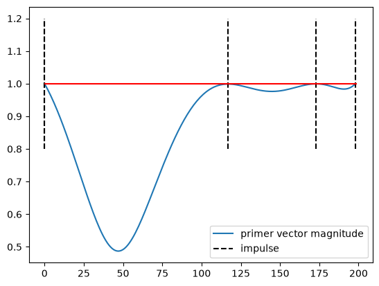
The very same trajectory is also studied in the notebook dedicated to the primer vector where the whole theory is also developed and coded as to show its inner workings.