Zero-Order Hold: TOPS problems I

This tutorial shows how to solve benchmark problems from the TOPS database (Trajectory Optimisation Problems in Space) using pykep wrappers based on the Zero-Order Hold (ZOH) transcription described in [IHA+26].

We focus on four benchmark families exposed in the gym module:

• pykep.trajopt.gym.tops_twobody (two-body, Cartesian state)

• pykep.trajopt.gym.tops_mee (two-body, modified equinoctial elements)

• pykep.trajopt.gym.tops_cr3bp (CR3BP)

• pykep.trajopt.gym.tops_ss (solar sailing)

All of them are Non-Linear Programming Problems, in a UDP format compatible with pygmo [BI20], and all follow the same workflow:

1. instantiate a TOPS benchmark wrapper,

2. build pg.problem,

3. verify analytical gradients against finite differences,

4. solve with IPOPT,

5. inspect the trajectory and controls.

For API details and background material, see:

• Trajectory optimization API

• TOPS benchmark overview

• Zero-Order Hold leg tutorial

Decision vectors and time encoding

The wrappers in this notebook are built on:

• pykep.trajopt.zoh_point2point (low-thrust)

• pykep.trajopt.zoh_ss_point2point (solar-sail)

For pykep.trajopt.zoh_point2point, the decision vector is:

\[ \mathbf{x} = [m_f] + [T_0, i_{x0}, i_{y0}, i_{z0}] + \cdots + [T_{N-1}, i_{x,N-1}, i_{y,N-1}, i_{z,N-1}] + [tof] (+ [w_0,\ldots,w_{N-1}]) \]

where:

• \(m_f\) is the final mass,

• \((T_k, i_{xk}, i_{yk}, i_{zk})\) is the segment thrust magnitude and direction,

• \(tof\) is total time of flight,

• \(w_k\) are optional softmax weights (only for time_encoding="softmax").

For pykep.trajopt.zoh_ss_point2point, the decision vector is:

\[ \mathbf{x} = [\alpha_0, \beta_0, \ldots, \alpha_{N-1}, \beta_{N-1}] + [tof] (+ [w_0,\ldots,w_{N-1}]) \]

where \((\alpha_k, \beta_k)\) are sail cone and clock angles (RTN frame) held constant on each segment.

Uniform vs softmax time grids

With time_encoding="uniform", segment durations are equal. With time_encoding="softmax", durations are learned via weights and satisfy positivity and partition of unity:

\[ \Delta t_k = tof\,\mathrm{softmax}(\mathbf{w})_k, \qquad t_{k+1}=t_k+\Delta t_k. \]

We start from a two-body Cartesian case and then repeat the same solver pipeline on MEE, CR3BP, and solar-sail dynamics.

This makes the notebook useful as both:

• a practical TOPS benchmark tutorial, and

• a template for your own ZOH-based optimization studies.

First, import the required packages.

# Core numerics, optimization, and plotting imports used throughout the tutorial
import pykep as pk 
import numpy as np
import pygmo as pg

from matplotlib import pyplot as plt

Configure the nonlinear optimizer.

We use IPOPT with strict tolerances so the gradient checks and feasibility status are meaningful when comparing benchmark instances.

# IPOPT reference setup used consistently across all TOPS sections
ipopt_integer_options = {
    "max_iter": 2000,
}
ipopt_numeric_options = {
    "tol": 1e-10,
}
ipopt_string_options = {
    "sb": "yes",
}

ipopt = pg.ipopt()
ipopt.set_integer_options(ipopt_integer_options)
ipopt.set_numeric_options(ipopt_numeric_options)
ipopt.set_string_options(ipopt_string_options)
algo = pg.algorithm(ipopt)

Two-body dynamics (Cartesian)

This section uses a TOPS two-body benchmark wrapped by pykep.trajopt.gym.tops_twobody.

Workflow:

1. load a named TOPS case (P0, P1, …),

2. build the pygmo problem and set feasibility tolerance,

3. verify analytical gradients,

4. solve with IPOPT and inspect mass / time-of-flight / geometry.

# 1) Select a TOPS benchmark case and build the wrapped UDP
prob_name = "P0"
udp = pk.trajopt.gym.tops_twobody(prob_name, nseg=10, time_encoding="uniform")
print(udp.extra_info)

# 2) Wrap into a pygmo problem and set feasibility tolerance for reporting
prob = pg.problem(udp)
prob.c_tol = 1e-7 # This affects pagmo feasibility checks, not IPOPT's internal tol

Mildly-elliptic to mildly-elliptic transfer (e_s~0.201, e_f~0.210) in fixed tof -> T=0.22N, Isp=3000s

Check analytical gradients against finite differences before optimization.

For these direct methods, this is a key reliability step: if this check is poor, solver behavior and convergence claims are not trustworthy.

# Compare analytical and finite-difference gradients at a random initial point
pop = pg.population(prob, 1)
grad_err = pg.estimate_gradient_h(udp.fitness, pop.champion_x, dx=1e-8) - udp.gradient(pop.champion_x)
grad_err.max(), grad_err.min()

(3.6446017148694665e-07, -2.7905344757161998e-07)

# Solve and report a compact set of diagnostics
pop = algo.evolve(pop)
print(prob.feasibility_f(pop.champion_f))
print("Objective:", pop.champion_f[0])
print("Final mass:", pop.champion_x[0] * udp.MASS)
print("Final tof:", pop.champion_x[4*udp.nseg+1] * udp.TIME)

True
Objective: -0.919693557939
Final mass: 0.919693557939
Final tof: 11.0

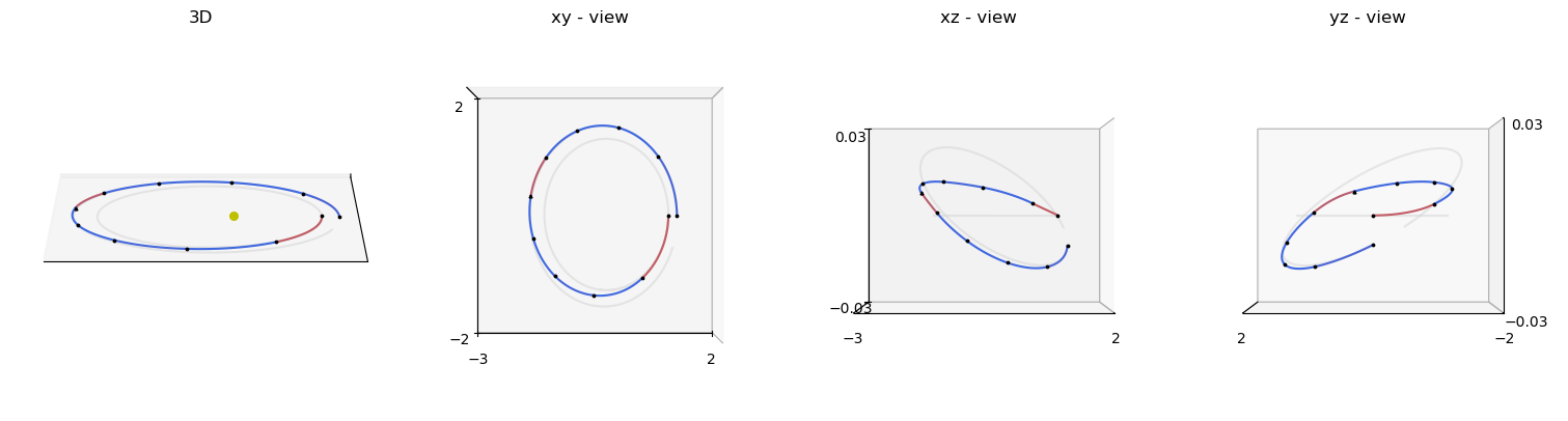
axes = udp.plot(pop.champion_x, N=100, mark_segments=True, s=3, c="k")

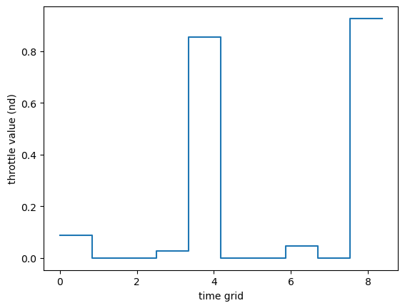
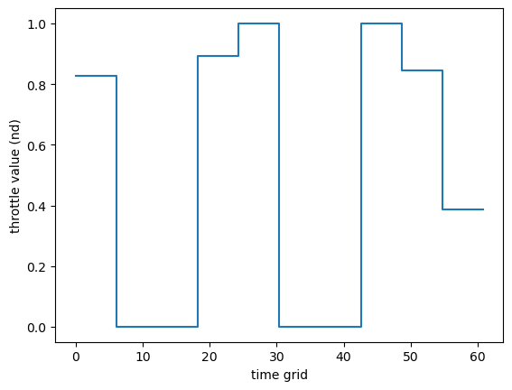
udp.plot_throttle(pop.champion_x)

<Axes: xlabel='time grid', ylabel='throttle value (nd)'>

Two-body dynamics (Modified Equinoctial Elements)

We now solve the MEE variant through pykep.trajopt.gym.tops_mee, reusing the exact same numerical pipeline.

Only the internal dynamics/state representation changes; the user-facing optimization workflow remains identical.

For element definitions and conversions, see Elements and conversions.

# 1) Load a TOPS MEE benchmark and inspect its metadata
prob_name = "P0"
udp = pk.trajopt.gym.tops_mee(prob_name, nseg=10, time_encoding="uniform")
print(udp.extra_info)

# 2) Create pygmo wrapper and harmonize feasibility tolerance across sections
prob = pg.problem(udp)
prob.c_tol = 1e-7 # This affects pagmo feasibility checks, not IPOPT's internal tol

Dionysus problem (doi: 10.2514/1.G000379) - Fixed time

# Gradient consistency check for the MEE benchmark
pop = pg.population(prob, 1)
grad_err = pg.estimate_gradient_h(udp.fitness, pop.champion_x, dx=1e-8) - udp.gradient(pop.champion_x)
grad_err.max(), grad_err.min()

(1.643901670478527e-06, -1.9111350484379841e-06)

# Solve and summarize
pop = algo.evolve(pop)
print(prob.feasibility_f(pop.champion_f))
print("Objective:", pop.champion_f[0])
print("Final mass:", pop.champion_x[0] * udp.MASS)
print("Final tof:", pop.champion_x[4*udp.nseg+1] * udp.TIME)

True
Objective: -0.589100288319
Final mass: 0.589100288319
Final tof: 60.7909197787

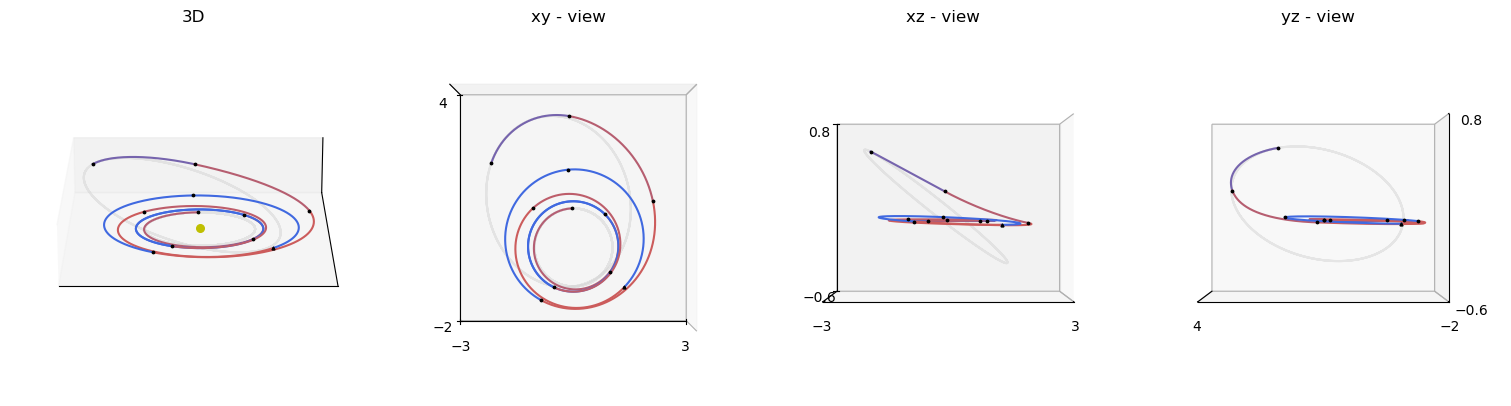
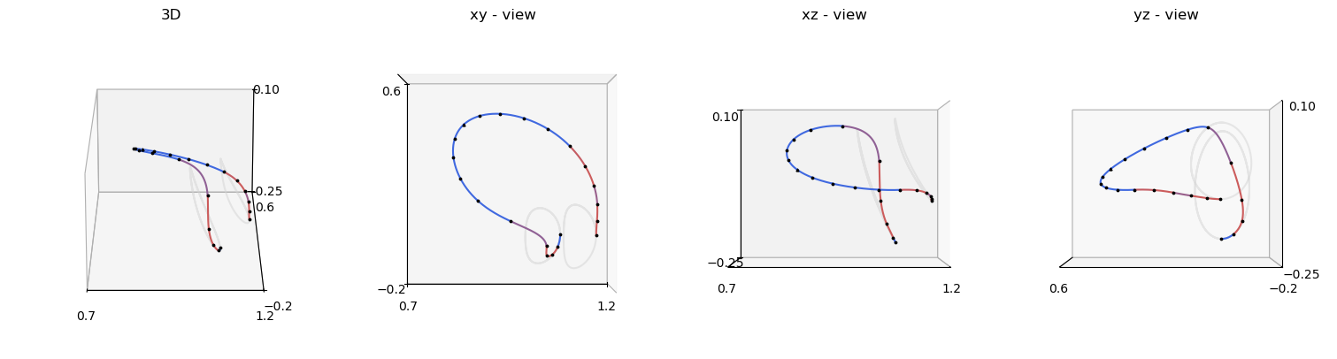
axes = udp.plot(pop.champion_x, N=300, mark_segments=True, s=3, c="k")

udp.plot_throttle(pop.champion_x)

<Axes: xlabel='time grid', ylabel='throttle value (nd)'>

Circular Restricted Three-Body Problem (CR3BP)

This section uses pykep.trajopt.gym.tops_cr3bp.

The wrapper configures the CR3BP-specific dynamics and parameters internally, while keeping the same optimizer and validation structure used in previous sections.

For model background, see CR3BP dynamics.

# 1) Load a TOPS CR3BP benchmark
prob_name = "P0"
udp = pk.trajopt.gym.tops_cr3bp(prob_name, nseg=20, time_encoding="uniform")
print(udp.extra_info)

# 2) Wrap for optimization
prob = pg.problem(udp)
prob.c_tol = 1e-7 # This affects pagmo feasibility checks, not IPOPT's internal tol

Halo 2 Halo in fixed tof

# Gradient consistency check for the CR3BP benchmark
pop = pg.population(prob, 1)
grad_err = pg.estimate_gradient_h(udp.fitness, pop.champion_x, dx=1e-8) - udp.gradient(pop.champion_x)
grad_err.max(), grad_err.min()

(1.4835070419449287e-06, -1.1432011767231742e-06)

# Solve and summarize
pop = algo.evolve(pop)
print(prob.feasibility_f(pop.champion_f))
print("Objective:", pop.champion_f[0])
print("Final mass:", pop.champion_x[0])
print("Final tof:", pop.champion_x[4*udp.nseg+1])

True
Objective: -0.946927194474
Final mass: 0.946927194474
Final tof: 5.0

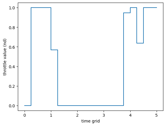
axes = udp.plot(pop.champion_x, N=1000, mark_segments=True, s=3, c="k")

udp.plot_throttle(pop.champion_x);

Solar-sail dynamics

Finally, we solve a TOPS solar-sail benchmark with pykep.trajopt.gym.tops_ss, internally based on pykep.trajopt.zoh_ss_point2point.

As above, we keep the same verification-and-solve protocol (gradient check, IPOPT solve, trajectory inspection), so results are directly comparable across dynamics.

For additional sail-leg details, see the Zero-Order Hold leg tutorial and Trajectory optimization API.

# 1) Load a TOPS solar-sail benchmark
prob_name = "P1"
udp = pk.trajopt.gym.tops_ss(prob_name, nseg=10, time_encoding="uniform")
print(udp.extra_info)

# 2) Build pygmo wrapper
prob = pg.problem(udp)
prob.c_tol = 1e-7 # This affects pagmo feasibility checks, not IPOPT's internal tol

Eccentric (e=0.5, a=2) to highly-eccentric (e=0.9, a=10) orbit at periapsis (rp=1, nd)

# Gradient consistency check for the solar-sail benchmark
pop = pg.population(prob, 1)
grad_err = pg.estimate_gradient_h(udp.fitness, pop.champion_x, dx=1e-8) - udp.gradient(pop.champion_x)
grad_err.max(), grad_err.min()

(1.6336881770939726e-05, -7.4573648817022331e-05)

# Solve and summarize (for zoh_ss_point2point, tof is the last decision variable)
pop = algo.evolve(pop)
print(prob.feasibility_f(pop.champion_f))
print("Objective:", pop.champion_f[0])
print("Final tof:", pop.champion_x[-1] * udp.TIME)

True
Objective: 180.0
Final tof: 180.0

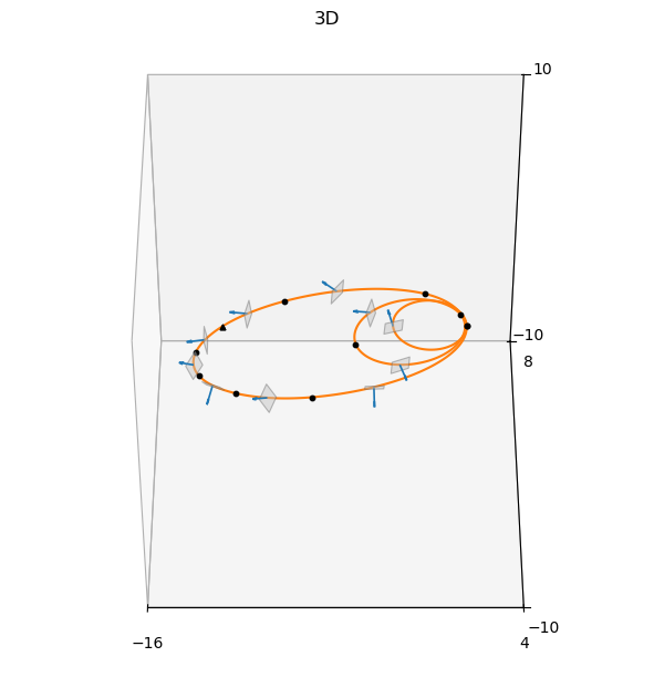
ax = udp.plot(pop.champion_x, N=100, mark_segments=True, sail_size=0.5, s=10, c='k')