Basic Multi-Objective Functionalities#
In this tutorial we will learn how to use pygmo to solve multiple-objective optimization problems. We assume that you already know how to write your own multi-objective problem (UDP) and will thus here focus on some added functionalities that are intended to facilitate the analysis of your problem.
Let us start to define our population:
>>> from pygmo import *
>>> udp = zdt(prob_id = 1)
>>> pop = population(prob = udp, size = 10, seed = 3453412)
We here make use of first problem of the ZDT benchmark suite implemented in zdt
and we create a population
containing 10 individuals randomly created within the box bounds. Which individuals belong to which non-dominated front?
We can immediately see this by running the fast non-dominated sorting algorithm fast_non_dominated_sorting():
>>> ndf, dl, dc, ndl = fast_non_dominated_sorting(pop.get_f())
[array([3, 4, 7, 8, 9], dtype=uint64), array([0, 5, 1, 6], dtype=uint64), array([2], dtype=uint64)]
A visualization of the different non-dominated fronts can also be easily obtained.
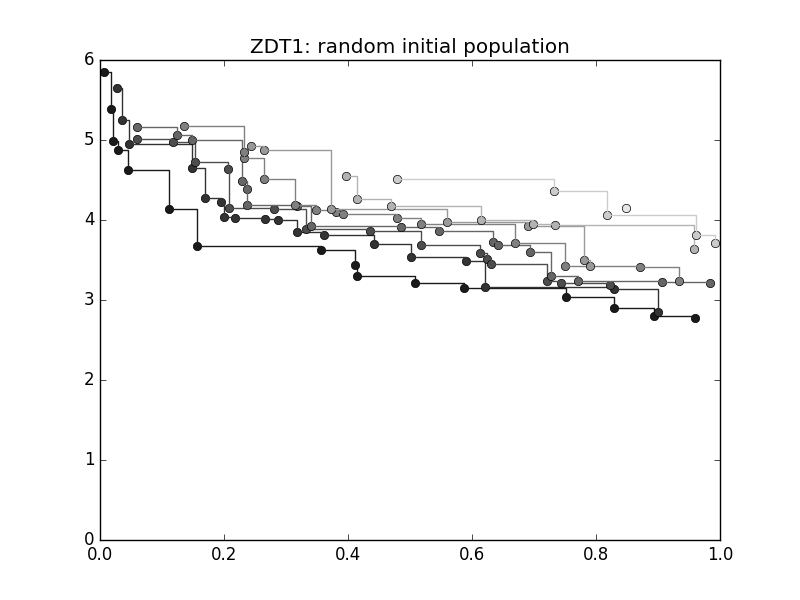
For example, generating a new population with 100 individuals:
>>> from matplotlib import pyplot as plt
>>> pop = population(udp, 100)
>>> ax = plot_non_dominated_fronts(pop.get_f())
>>> plt.ylim([0,6])
>>> plt.title("ZDT1: random initial population")
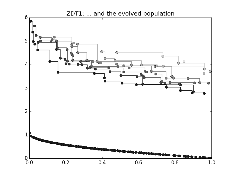
where each successive pareto front is plotted in darker colour. If we now type:
>>> algo = algorithm(moead(gen = 250))
>>> pop = algo.evolve(pop)
>>> ax = plot_non_dominated_fronts(pop.get_f())
>>> plt.title("ZDT1: ... and the evolved population")
we have instantiated the algorithm moead, able to tackle
multi-objective problems, fixing the number of generations to 250. In the following line we use directly
the method pygmo.moead.evolve() of the algorithm to evolve the population
The entire population is now on one non-dominated front as can be easily verified typing:
>>> ndf, dl, dc, ndl = fast_non_dominated_sorting(pop.get_f())
>>> print(ndf)
[array([ 0,  1,  2,  3,  4,  5,  6,  7,  8,  9, 10, 11, 12, 13, 14, 15, 16,
       17, 18, 19, 20, 21, 22, 23, 24, 25, 26, 27, 28, 29, 30, 31, 32, 33,
       34, 35, 36, 37, 38, 39, 40, 41, 42, 43, 44, 45, 46, 47, 48, 49, 50,
       51, 52, 53, 54, 55, 56, 57, 58, 59, 60, 61, 62, 63, 64, 65, 66, 67,
       68, 69, 70, 71, 72, 73, 74, 75, 76, 77, 78, 79, 80, 81, 82, 83, 84,
       85, 86, 87, 88, 89, 90, 91, 92, 93, 94, 95, 96, 97, 98, 99], dtype=uint64)]
The problems in the pygmo.zdt problem suite (as well as those in the pygmo.dtlz) have a nice convergence metric
implemented called p_distance. We can check how well the non dominated front is covering the known Pareto-front
>>> udp.p_distance(pop)
0.03926512747685471
If we are not happy on the value of such a metric, we can evolve the population for some more generations to improve the figure:
>>> pop = algo.evolve(pop)
>>> udp.p_distance(pop)
0.010346571321103046